A Python Package for Sampling from Copulae: clayton
A Python Package for Sampling from Copulae: clayton
ISSN 2824-7795
The package \textsf{clayton} is designed to be intuitive, user-friendly, and efficient. It offers a wide range of copula models, including Archimedean, Elliptical, and Extreme. The package is implemented in pure \textsf{Python}, making it easy to install and use.
The package \textsf{clayton} is designed to be intuitive, user-friendly, and efficient. It offers a wide range of copula models, including Archimedean, Elliptical, and Extreme. The package is implemented in pure \textsf{Python}, making it easy to install and use. In addition, we provide detailed documentation and examples to help users get started quickly. We also conduct a performance comparison with existing \textsf{R} packages, demonstrating the efficiency of our implementation. The \textsf{clayton} package is a valuable tool for researchers and practitioners working with copulae in \textsf{Python}.
1 Introduction
Modeling dependence relations between random variables is a topic of interest in probability theory and statistics. The most popular approach is based on the second moment of the underlying random variables, namely, the covariance. It is well known that only linear dependence can be captured by the covariance and it is only characteristic for a few models, e.g., the multivariate normal distribution or binary random variables. As a beneficial alternative to dependence, the concept of copulae, going back to Sklar (1959), has drawn a lot of attention. The copula C: [0,1]^d \rightarrow [0,1] of a random vector \mathbf{X} = (X_0, \dots, X_{d-1}) with d \geq 2 allows us to separate the effect of dependence from the effect of the marginal distribution, such that:
where (x_0, \dots, x_{d-1}) \in \mathbb{R}^d. The main consequence of this identity is that the copula completely characterizes the stochastic dependence between the margins of \mathbf{X}.
In other words, copulae allow us to model marginal distributions and dependence structure separately. Furthermore, motivated by Sklar’s theorem, the problem of investigating stochastic dependence is reduced to the study of multivariate distribution functions under the unit hypercube [0,1]^d with uniform margins. The theory of copulae has been of prime interest for many applied fields of science, such as quantitative finance (Patton (2012)) or environmental sciences (Mishra and Singh (2011)). This increasing number of applications has led to a demand for statistical methods. For example, semiparametric estimation (Genest, Ghoudi, and Rivest (1995)), nonparametric estimation (Fermanian, Radulović, and Wegkamp (2004)) of copulae or nonparametric estimation of conditional copulae (Gijbels, Omelka, and Veraverbeke (2015), Portier and Segers (2018)) have been investigated. These results are established for a fixed arbitrary dimension d \geq 2, but several investigations (e.g. Einmahl and Lin (2006), Einmahl and Segers (2021)) are done for functional data for the tail copula, which captures dependence in the upper tail.
Software implementation of copulae has been extensively studied in \textsf{R}, for example in the packages A. G. Stephenson (2002), Jun Yan (2007), Schepsmeier et al. (2019). However, methods for working with copulae in \textsf{Python} are still limited. As far as we know, copula-dedicated packages in \textsf{Python} are mainly designed for modeling, such as Alvarez et al. (2021) and Bock and Chapman (2021). These packages use maximum likelihood methods to estimate the copula parameters from observed data and generate synthetic data using the estimated copula model. Other packages provide sampling methods for copulae, but they are typically restricted to the bivariate case and the conditional simulation method (see, for example, Baudin et al. (2017)). Additionally, if the multivariate case is considered only Archimedean and elliptical copulae are under interest and those packages (see Nicolas (2022)) do not include the extreme value class in arbitrary dimensions d \geq 2. In this paper, we propose to implement a wide range of copulae, including the extreme value class, in arbitrary fixed dimension d \geq 2.
Through this paper we adopt the following notational conventions: all the indices will start at 0 as in \textsf{Python}. Consider (\Omega, \mathcal{A}, \mathbb{P}) a probability space and let \textbf{X} = (X_0, \dots, X_{d-1}) be a d-dimensional random vector with values in (\mathbb{R}^d, \mathcal{B}(\mathbb{R}^d)), with d \geq 2 and \mathcal{B}(\mathbb{R}^d) the Borel \sigma-algebra of \mathbb{R}^d. This random vector has a joint distribution F with copula C and its margins are denoted by F_j(x) = \mathbb{P}\{X_j \leq x\} for all x \in \mathbb{R} and j \in \{0, \dots, d-1\}. Denote by \textbf{U} = (U_0, \dots, U_{d-1}) a d random vector with copula C and uniform margins. All bold letters \textbf{x} will denote a vector of \mathbb{R}^d.
The \textsf{clayton} package, whose Python code can be found in https://github.com/Aleboul/clayton, uses object-oriented features of the Python language. The package contains classes for Archimedean, elliptical, and extreme value copulae. In Section 2, we briefly describe the classes defined in the package. Section 3 presents methods for generating random vectors. In Section 4, we apply the \textsf{clayton} package to model pairwise dependence between maxima. Section 5 discusses potential improvements to the package and provides concluding remarks. Sections from Section 6.1 to Section 6.5 define and illustrate all the parametric copula models implemented in the package.
2 Classes
Figure 1: The figure shows a object diagram that structures the code. The \textbf{Multivariate} class serves as the root and is used to instantiate all its child classes \textbf{Archimedean}, \textbf{Extreme}, \textbf{Gaussian}, and \textbf{Student} in red. The blue-colored classes correspond to various parametric copula models, and the green-colored classes represent examples of methods. Symbols \varphi, \varphi^\leftarrow, \dot{\varphi} correspond to the generator function, its inverse, and its derivative, respectively, while A, \dot{A} refer to the Pickands dependence function and its derivative.
The architecture of the code is shown in Figure 1. At the third level of the architecture, we find important parametric models of Archimedean and extreme value copulae (depicted as blue in the figure). These parametric models contain methods such as the generator function \varphi (see Section 2.1) for Archimedean copulae and the Pickands dependence function A (see Section 2.2) for extreme value copulae (depicted as green in the figure). We provide a brief overview of Archimedean copulae and some of their properties in high-dimensional spaces in Section 2.1. A characterization of extreme value copulae is given in Section 2.2. The from Section 6.1 to Section 6.5 define and illustrate all the copula models implemented in the package.
2.1 The Archimedean class
Let \varphi be a generator that is a strictly decreasing, convex function from [0,1] to [0, \infty] such that \varphi(1) = 0 and \varphi(0) = \infty. We denote the generalized inverse of \varphi by \varphi^\leftarrow. Consider the following equation:
If this relation holds and C is a copula function, then C is called an Archimedean copula. A necessary condition for Equation 1 to be a copula is that the generator \varphi is a d-monotonic function, i.e., it is differentiable up to the order d and its derivatives satisfy
for x \in (0, \infty) (see Corollary 2.1 of McNeil and Nešlehová (2009)). Note that d-monotonic Archimedean inverse generators do not necessarily generate Archimedean copulae in dimensions higher than d (see McNeil and Nešlehová (2009)). As a result, some Archimedean subclasses are only implemented for the bivariate case as they do not generate an Archimedean copula in higher dimensions. In the bivariate case, Equation 2 can be interpreted as \varphi being a convex function.
The \textsf{clayton} package implements common one-parameter families of Archimedean copulae, such as the Clayton (Clayton (1978)), Gumbel (Gumbel (1960)), Joe (Joe (1997)), Frank (Frank (1979)), and AMH (Ali, Mikhail, and Haq (1978)) copulae for the multivariate case. It is worth noting that all Archimedean copulae are symmetric, and in dimensions 3 or higher, only positive associations are allowed. For the specific bivariate case, the package also implements other families, such as those numbered from 4.2.9 to 4.2.15 and 4.2.22 in Section 4.2 of Nelsen (2007). Definitions and illustrations of these parametric copula models can be found in Section 6.1 and Section 6.3.
2.2 The Extreme class
Investigating the notion of copulae within the framework of multivariate extreme value theory leads to the extreme value copulae (see Gudendorf and Segers (2010) for an overview) defined as
C(\textbf{u}) = \exp \left( - \ell(-\ln(u_0), \dots, -\ln(u_{d-1})) \right), \quad \textbf{u} \in (0,1]^d,
\tag{3} where \ell: [0,\infty)^d \rightarrow [0,\infty) the stable tail dependence function which is convex, homogeneous of order one, namely \ell(c\textbf{x}) = c \ell(\textbf{x}) for c > 0 and satisfies \max(x_0,\dots,x_{d-1}) \leq \ell(x_0,\dots,x_{d-1}) \leq x_0+\dots+x_{d-1}, \forall \textbf{x} \in [0,\infty)^d. Let \Delta^{d-1} = \{\textbf{w} \in [0,1]^d: w_0 + \dots + w_{d-1} = 1\} be the unit simplex. The Pickands dependence function A: \Delta^{d-1} \rightarrow [1/d,1] characterizes \ell by its homogeneity, which is the restriction of \ell to the unit simplex \Delta^{d-1}:
\ell(x_0, \dots,x_{d-1}) = (x_0 + \dots + x_{d-1}) A(w_0, \dots, w_{d-1}), \quad w_j = \frac{x_j}{x_0 + \dots + x_{d-1}},
\tag{4} for j \in \{1,\dots,d-1\} and w_0 = 1 - w_1 - \dots - w_{d-1} with \textbf{x} \in [0, \infty)^d \setminus \{\textbf{0}\}. The Pickands dependence function characterizes the extremal dependence structure of an extreme value random vector and verifies \max\{w_0,\dots,w_{d-1}\} \leq A(w_0,\dots,w_{d-1}) \leq 1 where the lower bound corresponds to comonotonicity and the upper bound corresponds to independence. Estimating this function is an active area of research, with many compelling studies having been conducted on the topic (see, for example, Bücher, Dette, and Volgushev (2011), Gudendorf and Segers (2012)).
From a practical point of view, the family of extreme value copulae is very rich and arises naturally as the limiting distribution of properly normalised componentwise maxima. Furthermore, it contains a rich variety of parametric models and allows asymmetric dependence, that is, for the bivariate case:
\exists (u_0,u_1) \in [0,1]^2, \quad C(u_0,u_1) \neq C(u_1,u_0).
In the multivariate framework, the logistic copula (or Gumbel, see Gumbel (1960)), the asymmetric logistic copula (Tawn (1990)), the Hüsler and Reiss distribution (Hüsler and Reiss (1989)), the t-EV copula (Demarta and McNeil (2005)), Bilogistic model (Smith (1990)) are implemented. It’s worth noting that the logistic copula is the sole model that is both Archimedean and extreme value. The library includes bivariate extreme value copulae such as asymmetric negative logistic (Joe (1990)), asymmetric mixed (Tawn (1988)). The reader is again invited to read from Section 6.2 to Section 6.4 for precise definitions of these models.
3 Random number generator
We propose a \textsf{Python}-based implementation for generating random numbers from a wide variety of copulae. The \textsf{clayton} package requires a few external libraries that are commonly used in scientific computing in \textsf{Python}.
numpy version 1.6.1 or newer. This is the fundamental package for scientific computing, it contains linear algebra functions and matrix / vector objects (Harris et al. (2020)).
scipy version 1.7.1 or newer. A library of open-source software for mathematics, science and engineering (Virtanen et al. (2020)).
The \textsf{clayton} package provides two methods for generating random vectors: \texttt{sample\_unimargin} and \texttt{sample}. The first method generates a sample where the margins are uniformly distributed on the unit interval [0,1], while the second method generates a sample from the chosen margins.
In Section 3.1, we present an algorithm that uses the conditioning method to sample from a copula. This method is very general and can be used for any copula that is sufficiently smooth (see Equation 5 and Equation 8 below). However, the practical infeasibility of the algorithm in dimensions higher than 2 and the computational intensity of numerical inversion call for more efficient ways to sample in higher dimensions. The purpose of Section 3.2 is to present such methods and to provide details on the methods used in the \textsf{clayton} package. In each section, we provide examples of code to illustrate how to instantiate a copula and how to sample with \textsf{clayton}.
In the following sections, we will use \textsf{Python} code that assumes that the following packages have been loaded:
Hide/Show the code
import claytonfrom clayton.rng import base, evd, archimedean, monte_carloimport numpy as npimport seaborn as snsimport matplotlib.pyplot as pltfrom scipy.stats import norm, exponplt.style.use('qb-light.mplstyle') # for fancy figuresnp.random.seed(10)
3.1 The bivariate case
In this subsection, we address the problem of generating a bivariate sample from a specified joint distribution with d=2. Suppose that we want to sample a bivariate random vector \textbf{X} with copula C. In the case where the components are independent, the sampling procedure is straightforward: we can independently sample X_0 and X_1. However, in the general case where the copula is not the independent copula, this approach is not applicable.
One solution to this problem is to use the conditioning method to sample from the copula. This method relies on the fact that given (U_0, U_1) with copula C, the conditonal law of U_1 given U_0 is written as:
This allows us to first sample U_0 from a uniform distribution on the unit interval, and then to use the copula to generate U_1 given U_0. Finally, we can transform the resulting sample (U_0, U_1) into the original space by applying the inverse marginal distributions F_0^{-1} and F_1^{-1} to U_0 and U_1 respectively. Thus, an algorithm for sampling bivariate copulae is given in Figure 2. Algorithm in Figure 2 presents a procedure for generating a bivariate sample from a copula. The algorithm takes as input the length of the sample n, as well as the parameters of the copula (\theta, \psi_1, \psi_2). The output is a bivariate sample from the desired copula model, denoted \{(u_0^{(1)},u_1^{(1)}), \dots, (u_0^{(n)},u_1^{(n)})\}. This algorithm is applicable as long as the copula has a first partial derivative with respect to its first component.
Figure 2: Conditional sampling from copula
For step 6 of the algorithm, we need to find u_1 \in [0,1] such that c_{u_0}(u_1) - t_1 = 0 holds. This u_1 always exists because for every u \in ]0,1[, we have 0 \leq c_{u_0}(u) \leq 1, and the function u \mapsto c_{u_0}(u) is increasing (see Theorem 2.2.7 of Nelsen (2007) for a proof). This step can be solved using the function from the package. A sufficient condition for a copula to have a first partial derivative with respect to its first component in the Archimedean and extreme value cases is that the generator \varphi and the Pickands dependence function A are continuously differentiable on ]0,1[, respectively. In this case, the first partial derivatives of the copula are given by:
where t = \ln(u_1) / \ln(u_0u_1) \in (0,1) and \mu(t) = A(t) - tA'(t).
We now have all the necessary theoretical tools to give details on how the \textsf{clayton} package is designed. The file \texttt{base.py} contains the \textbf{Multivariate} class and the \texttt{sample} method to generate random numbers from \textbf{X} with copula C. To do so, we use the inversion method that is to sample from \textbf{U} using algorithm in Figure 2 and we compose the corresponding uniform margins by F_j^\leftarrow. indicates that the sole knowledge of A and \varphi and their respective derivatives are needed in order to perform the sixth step of algorithm in Figure 2. For that purpose, \texttt{cond\_sim} method located inside \textbf{Archimedean} and \textbf{Extreme} classes performs algorithm in Figure 2. Then each child of the bivariate \textbf{Archimedean} (resp. \textbf{Extreme}) class is thus defined by its generator \varphi (resp. A), it’s derivative \varphi' (resp. A') and it’s inverse \varphi^\leftarrow as emphasized in green in Figure 1. Namely, we perform algorithm in Figure 2 for the \textbf{Archimedean} subclasses \texttt{Frank}, \texttt{AMH}, \texttt{Clayton} (when \theta < 0 for the previous three), \texttt{Nelsen\_9}, \texttt{Nelsen\_10}, \texttt{Nelsen\_11}, \texttt{Nelsen\_12}, \texttt{Nelsen\_13}, \texttt{Nelsen\_14}, \texttt{Nelsen\_15} and \texttt{Nelsen\_22}. For the \textbf{Extreme} class, such algorithm is performed for the \texttt{AsyNegLog} and \texttt{AsyMix}. For other models, faster algorithms are known and thus implemented, we refer to Section 3.2 for details.
The following code illustrates the random vector generation for a bivariate Archimedean copula. By defining the parameter of the copula and the sample’s length, the constructor for this copula is available and can be called using the \texttt{Clayton} method, such as:
To obtain a sample with uniform margins and a Clayton copula, we can use the \texttt{sample\_unimargin} method, as follows:
Hide/Show the code
sample = copula.sample_unimargin()
Here, the \texttt{sample} object is a \textsf{numpy} array with 2 columns and 1024 rows, where each row contains a realization from a Clayton copula (see below)
We will now address the generation of multivariate Archimedean and Extreme value copulae proposed in the Clayton package. In the multivariate case, the link between partial derivatives and the conditional law remains. Indeed, let (U_0, \dots, U_{d-1}) be a d-dimensional random vector with uniform margins and copula C. The conditional distribution of U_k given the values of U_0, \dots, U_{k-1} is
for k \in {1,\dots, d-1}. The conditional simulation algorithm may be written as follows.
Generate d independent uniform random on [0,1] variates v_0, \dots, v_{d-1}.
Set u_0 = v_0.
For k = 1, \dots, d-1, evaluate the inverse of the conditional distribution given by at v_k, to generate u_k.
Nevertheless, the evaluation of the inverse conditional distribution becomes increasingly complicated as the dimension d increases. Furthermore, it can be difficult for some models to derive a closed form of Equation 8 that makes it impossible to implement it in a general algorithm with only the dimension d as an input. For multivariate Archimedean copulae, McNeil and Nešlehová (2009) give a method to generate a random vector from the d-dimensional copula C with generator \varphi (see Section 5.2 of McNeil and Nešlehová (2009)). A stochastic representation for Archimedean copulae generated by a d-monotone generator is given by
where R \sim F_R, the radial distribution which is independent of S and S is distributed uniformly in the unit simplex \Delta^{d-1}. One challenging aspect of this algorithm is to have an accurate evaluation of the radial distribution of the Archimedean copula and thus to numerically inverse this distribution. The associated radial distribution for the \textsf{Clayton} copula is given in Example 3.3 McNeil and Nešlehová (2009) while those of the \textsf{Joe}, \textsf{AMH}, \textsf{Gumbel} and \textsf{Frank} copulae are given in Hofert, Mächler, and McNeil (2012). In general, one can use numerical inversion algorithms for computing the inverse of the radial distribution, however it will lead to spurious numerical errors. Other algorithms exist when the generator is known to be the Laplace-Stieltjes transform, denoted as \mathcal{LS}, of some positive random variables (see Marshall and Olkin (1988), Frees and Valdez (1998)). This positive random variable is often referenced as the frailty distribution. In this framework, Archimedean copulae allow for the stochastic representation
with V \sim F = \mathcal{LS}^{-1}[\varphi^\leftarrow] the frailty and E_1, \dots, E_d are distributed i.i.d. according to a standard exponential and independent of V. Algorithm in Figure 3 presents a procedure for generating a multivariate sample from an Archimedean copula where the frailty distribution is known. The algorithm takes as an input the length of the sample n, as well as the parameter of the copula \theta. The output is a d-variate sample from the desired copula model, denoted \{(u_0^{(1)}, \dots, u_{d-1}^{(1)}), \dots, (u_0^{(n)},\dots,u_{d-1}^{(n)})\}.
Figure 3: Sampling from Archimedean copula using frailty distribution
In this framework, we define \texttt{\_frailty\_sim} method defined inside the \textbf{Archimedean} class which performs algorithm in Figure 3. Then, each Archimedean copula is defined by the generator \varphi, it’s inverse \varphi^\leftarrow and the frailty distribution denoted as \mathcal{LS}^{-1}[\varphi^\leftarrow] as long as we know the frailty. This is the case for \texttt{Joe}, \texttt{Clayton}, \texttt{AMH} or \texttt{Frank}.
For the extreme value case, algorithms have been proposed, as in A. Stephenson (2003) (see Algorithms 2.1 and 2.2), who proposes sampling methods for the Gumbel and the asymmetric logistic model. These algorithms are implemented in the \textsf{clayton} package. Note that these algorithms are model-specific, thus the \texttt{sample\_unimargin} method is exceptionally located in the corresponding child of the multivariate \textbf{Extreme} class. Another procedure designed by Dombry, Engelke, and Oesting (2016) to sample from multivariate extreme value models using extremal functions (see Algorithm 2 in Dombry, Engelke, and Oesting (2016)) is also of prime interest. For the implemented models using this algorithm, namely \textbf{Hüsler-Reiss}, \textbf{tEV}, \textbf{Bilogistic} and \textbf{Dirichlet} models, a method called \texttt{\_rextfunc} is located inside each classes which allows to generate an observation from the according law of the extremal function.
Samples from the Gaussian and Student copula are directly given by Algorithm 5.9 and 5.10 respectively of Alexander J. McNeil (2005). As each algorithm is model specific, the \texttt{sample\_unimargin} method is located inside the \textbf{Gaussian} and \textbf{Student} classes.
We present how to construct a multivariate Archimedean copula and to generate random vectors from this model. Introducing the parameters of the copula, we appeal the following lines to construct our copula object:
4 Case study : Modeling pairwise dependence between spatial maximas with missing data
We now proceed to a case study where we use our package to assess, under a finite sample framework, the asymptotic properties of an estimator of the \lambda-madogram when data are completely missing at random (MCAR). This case study comes from numerical results of Boulin et al. (2022). The \lambda-madogram belongs to a family of estimators, namely the madogram, which is of prime interest in environmental sciences, as it is designed to model pairwise dependence between maxima in space, see, e.g., Bernard et al. (2013), Bador et al. (2015), Saunders, Stephenson, and Karoly (2021) where the madogram was used as a dissimilarity measure to perform clustering. Where in several fields, for example econometrics (Wooldridge (2007)) or survey theory (Boistard, Chauvet, and Haziza (2016)), the MCAR hypothesis appears to be a strong hypothesis, this hypothesis is more realistic in environmental research as the missingness of one observation is usually due to instruments, communication and processing errors that may be reasonably supposed independent of the quantity of interest. In Section 4.1, we define objects and properties of interest while in Section 4.2 we describe a detailed tutorial in \textsf{python} and with \textsf{clayton} package to compare the asymptotic variance with an empirical counterpart of the \lambda-madogram with \lambda = 0.5.
4.1 Background
It was emphasized that the possible dependence between maxima can be described with the extreme value copula. This function is completely characterized by the Pickands dependence function (see Equation 4) where the latter is equivalent to the \lambda-madogram introduced by Naveau et al. (2009) and defined as
with \lambda \in (0,1), and if \lambda = 0 and 0<u<1, then u^{1/\lambda} = 0 by convention. The \lambda-madogram took its inspiration from the extensively used geostatistics tool, the variogram (see Chapter 1.3 of Gaetan and Guyon (2008) for a definition and some classical properties). The \lambda-madogram can be interpreted as the L_1-distance between the uniform margins elevated to the inverse of the corresponding weights \lambda and 1-\lambda. This quantity describes the dependence structure between extremes by its relation with the Pickands dependence function. If we suppose that C is an extreme value copula as in , we have
with c(\lambda) = 2^{-1} (\lambda / (1-\lambda) + (1-\lambda)/\lambda) (see Proposition 3 of Marcon et al. (2017) for details).
We consider independent and identically distributed i.i.d. copies \textbf{X}_1, \dots, \textbf{X}_n of \textbf{X}. In presence of missing data, we do not observe a complete vector \textbf{X}_i for i \in \{1,\dots,n\}. We introduce \textbf{I}_i \in \{0,1\}^2 which satisfies, \forall j \in \{0,1\}, if X_{i,j} is not observed then I_{i,j} = 0. To formalize incomplete observations, we introduce the incomplete vector \tilde{\textbf{X}}_i with values in the product space \bigotimes_{j=1}^2 (\mathbb{R} \cup \{\textsf{NA}\}) such as
(\textbf{I}_i, \tilde{\textbf{X}}_i), \quad i \in \{1,\dots,n\},
\tag{12}
i.e. at each i \in \{1,\dots,n\}, several entries may be missing. We also suppose that for all i \in \{1, \dots,n \}, \textbf{I}_{i} are i.i.d copies from \textbf{I} = (I_0, I_1) where I_j is distributed according to a Bernoulli random variable \mathcal{B}(p_j) with p_j = \mathbb{P}(I_j = 1) for j \in \{0,1\}. We denote by p the probability of observing completely a realization from \textbf{X}, that is p = \mathbb{P}(I_0=1, I_1 = 1). In Boulin et al. (2022), hybrid and corrected estimators, respectively denoted as \hat{\nu}_n^{\mathcal{H}} and \hat{\nu}_n^{\mathcal{H*}}, are proposed to estimate nonparametrically the \lambda-madogram in presence of missing data completely at random. Furthermore, a closed expression of their asymptotic variances for \lambda \in ]0,1[ is also given. This result is summarized in the following proposition.
Theorem 1 (Boulin et al. (2022)) Let (\textbf{I}_i, \tilde{\textbf{X}_i})_{i=1}^n be a samble given by Equation 12. For \lambda \in ]0,1[, if C is an extreme value copula with Pickands dependence function A, we have as n \rightarrow \infty\begin{align*}
&\sqrt{n} \left(\hat{\nu}_n^{\mathcal{H}}(\lambda) - \nu( \lambda)\right) \overset{d}{\rightarrow} \mathcal{N}\left(0, \mathcal{S}^{\mathcal{H}}(p_1,p_2,p, \lambda)\right), \\
&\sqrt{n} \left(\hat{\nu}_n^{\mathcal{H}*}(\lambda) - \nu( \lambda)\right) \overset{d}{\rightarrow} \mathcal{N}\left(0, \mathcal{S}^{\mathcal{H}*}(p_1,p_2,p, \lambda)\right),
\end{align*}
where \mathcal{S}^{\mathcal{H}}(p_1,p_2,p, \lambda) and \mathcal{S}^{\mathcal{H}*}(p_1,p_2,p, \lambda) are the asymptoptic variances of the random variables.
4.2 Numerical results
Benefiting from generating data with \textsf{clayton} we are thus able, with Monte Carlo simulation, to assess theoretical results given by Theorem 1 in a finite sample setting. For that purpose, we implement a \textsf{MonteCarlo} class (in \texttt{monte\_carlo.py} file) which contains some methods to perform some Monte Carlo iterations for a given extreme value copula. Now, we set up parameters to sample our bivariate dataset. For this subsection, we choose the asymmetric negative logistic model (see Section 6.2 for a definition) with parameters \theta = 10, \psi_1 = 0.1, \psi_2 = 1.0 and we define the following function:
The 1024 \times 2 array \texttt{sample} contains 1024 realization of the \textbf{asymmetric negative logistic} model where the first column is distributed according to a standard normal random variable and the second column as a standard exponential. This distribution is depicted below. To obtain it, one needs the following lines of command:
Before going into further details, we will present the missing mechanism. Let V_0 and V_1 be random variables uniformly distributed under the ]0,1[ segment with copula C_{(V_0,V_1)}. We set I_0 = 1\{{V_0 \leq p_0}\} and I_1 = 1\{{V_1 \leq p_1}\}. It is thus immediate that I_0 \sim \mathcal{B}(p_0) and I_1 \sim \mathcal{B}(p_1) and p \triangleq \mathbb{P}\{I_0 = 1, I_1 =1 \} = C_{(V_0,V_1)}(p_0, p_1). For our illustration, we will take C_{(V_0,V_1)} as a copula with parameter \theta = 2.0 (we refer to Section 6.1 for a definition of this copula). For this copula, it is more likely to observe a realization v_0 \geq 0.8 from V_0 if v_1 \geq 0.8 from V_1. If we observe v_1 < 0.8, the realization v_0 is close to being independent of v_1. In climate studies, extreme events could damage the recording instrument in the surrounding regions where they occur, thus the missingness of one variable may depend on others. We initialize the copula C_{(V_0,V_1)} with the following line:
For a given \lambda \in ]0,1[, we now want to estimate a \lambda-madogram with a sample from the asymmetric negative logistic model, where some observations are missing due to the missing mechanism described above. We will repeat this step several times to compute an empirical counterpart of the asymptotic variance. The object has been designed for this purpose: we specify the number of iterations n_{iter} (take n_{iter} = 1024), the chosen extreme value copula (asymmetric negative logistic model), the missing mechanism (described by C_{(V_0,V_1)} and p_0 = p_1 = 0.9), and \lambda (noted \texttt{w}). We can write the following lines of code:
Hide/Show the code
u = np.array([0.9, 0.9]) n_iter, P, w =256, [[u[0], copula_miss._c( u)], [copula_miss._c(u), u[1]]], np.array([0.5,0.5]) monte = monte_carlo.MonteCarlo(n_iter=n_iter, n_samples=n_samples, copula=copula, copula_miss=copula_miss, weight=w, matp=P)
The \texttt{MonteCarlo} object is thus initialized with all parameters needed. We may use the \texttt{simu} method to generate a \texttt{DataFrame} (a \texttt{pandas} object) composed out 1024 rows and 3 columns. Each row contains an estimate of the \lambda-madogram, \hat{\nu}_n^{\mathcal{H}*} in Theorem 1 (\texttt{var\_mado}), the sample length n (\texttt{n}) and the normalized estimation error (\texttt{scaled}). We thus call the \texttt{simu} method.
The argument \texttt{corr=True} specifies that we compute the corrected estimator, \hat{\nu}_n^{\mathcal{H}*} in Theorem 1. Now, using the \texttt{var\_mado} method defined inside in the Extreme class, we obtain the asymptotic variance for the given model and parameters from the missing mechanism. We obtain this quantity as follows
We propose here to check numerically the asymptotic normality with variance \mathcal{S}^{\mathcal{H}*} of the normalized estimation error of the corrected estimator. We have all data in hand and the asymptotic variance was computed by lines above. We thus write:
5.1 Comparison of \textsf{clayton} with \textsf{R} packages
To compare to existing packages in \textsf{R}, we consider the \textsf{copula} package (Kojadinovic and Yan (2010)) and \textsf{mev} (Belzile et al. (2022)) for sampling from Archimedean and multivariate extreme value distributions, respectively. To run the experiment, we use two computer clusters. The first cluster consists of five nodes, each with two 18-core Xeon Gold 3.1 GHz processors and 192 GB of memory, with 2933 MHz per socket. The second cluster has two CPU sockets, each containing a Xeon Platinum 8268 2.90 GHz processor with 24 cores. These configurations provide a significant amount of computational power and are well-suited for handling complex, data-intensive tasks. We use the first cluster to install the \textsf{copula} package and sample from the \textbf{Clayton}, \textbf{Frank}, and \textbf{Joe} models. We consider an increasing dimension d \in \{50, 100, \dots, 1600\} for a fixed sample size of n=1000. For the copula package, we compute the average time spent across 100 runs in order to cancel out variability. We use the second cluster to install the \textsf{mev} package and call some of its methods to sample from the \textbf{Husler Reiss}, \textbf{Logistic}, and \textbf{TEV} distributions. Sampling from the latter is fast, but sampling from the two others is time consuming. Therefore, we only consider dimensions d \in \{25, 50, \dots, 250\} for a fixed sample size of n=1000.
Archimedean
Multivariate extreme value
Figure 4: Comparison results. Time spent (in seconds) to sample from the corresponding models with respect to the dimension d. The left panel shows the results for sampling from \textbf{Clayton}, \textbf{Frank} and \textbf{Joe} using \textsf{clayton} in \textsf{Python} and \textsf{copula} in \textsf{R}. The right panel shows the results for sampling from \textbf{HuslerReiss}, \textbf{Logistic} and \textbf{TEV} by \textsf{clayton} in \textsf{Python} and \textsf{mev} in \textsf{R}. In both cases, 1000 vectors are generated for each model.
The figure shows the results of a comparison between the \textsf{clayton} and \textsf{copula} packages in \textsf{R}, and the \textsf{mev} package in \textsf{Python}. The comparison shows that the \textsf{clayton} package is more efficient at sampling from \textbf{Clayton}, \textbf{Frank} and \textbf{Joe} copulae than the \textsf{copula} package. The gap in efficiency may be due to the choice of algorithms used in the \textsf{clayton} package, which uses frailty distributions. The time required for sampling increases linearly with the dimension for the \textsf{clayton} package, but shows a more erratic behavior for the \textsf{copula} package.
5.2 Conclusion
This paper presents the construction and some implementations of the \textsf{Python} package \textsf{clayton} for random copula sampling. This is a seminal work in the field of software implementation of copula modeling in \textsf{Python} and there is much more potential for growth. It is hoped that the potential diffusion of the software through those who need it may bring further implementations for multivariate modeling with copulae under \textsf{Python}. For example, choosing a copula to fit the data is an important but difficult problem. A robust approach to estimating copulae has been investigated recently by Alquier et al. (2022) using Maximum Mean Discrepancy. In relation to our example, semiparametric estimation of copulae with missing data could be of great interest, as proposed by Hamori, Motegi, and Zhang (2019).
Additionally, implementation of the algorithm proposed by McNeil and Nešlehová (2009) for generating random vectors for Archimedean copulae has been tackled, but as expected, numerical inversion gives spurious results, especially when the parameter \theta and the dimension d are high. Furthermore, as the support of the radial distribution is contained in the real line, numerical inversion leads to increased computational time. Further investigation is needed in order to generate random vectors from classical Archimedan models using the radial distribution.
A direction of improvement for the \textsf{clayton} package is dependence modeling with Vine copulae, which have recently been a tool of high interest in the machine learning community (see, e.g., Lopez-Paz, Hernández-Lobato, and Zoubin (2013), Veeramachaneni, Cuesta-Infante, and O’Reilly (2015), Carrera, Santana, and Lozano (2016), Gonçalves, Von Zuben, and Banerjee (2016) or Sun, Cuesta-Infante, and Veeramachaneni (2019)). This highlights the need for dependence modeling with copulae in \textsf{Python}, as a significant part of the machine learning community uses this language. In relation to this paper, Vine copulae may be useful for modeling dependencies between extreme events, as suggested by Simpson, Wadsworth, and Tawn (2021), Nolde and Wadsworth (2021). Furthermore, other copula models could be implemented to model further dependencies. These implementations will expand the scope of dependence modeling with \textsf{Python} and provide high-quality, usable tools for anyone who needs them.
References
Alexander J. McNeil, Paul Embrechts, Rudiger Frey. 2005. Quantitative Risk Management - Concepts, Techniques and Tools. Princeton Series in Finance. Princeton University Press. libgen.li/file.php?md5=478a0059673fecd0c76229cd3d8884e7.
Ali, Mir M, N. N Mikhail, and M.Safiul Haq. 1978. “A Class of Bivariate Distributions Including the Bivariate Logistic.”Journal of Multivariate Analysis 8 (3): 405–12. https://doi.org/https://doi.org/10.1016/0047-259X(78)90063-5.
Alquier, Pierre, Badr-Eddine Chérief-Abdellatif, Alexis Derumigny, and Jean-David Fermanian. 2022. “Estimation of Copulas via Maximum Mean Discrepancy.”Journal of the American Statistical Association, 1–16.
Alvarez, M., C. Sala, Y. Sun, J. D. Pérez, K. A. Zhang, A. Montanez, G. Bonomi, K. Veeramachaneni, I. Ramírez, and F. A. Hofman. 2021. “Copulas.”GitHub Repository. https://github.com/sdv-dev/Copulas; GitHub.
Bador, Margot, Philippe Naveau, Eric Gilleland, Mercè Castellà, and Tatiana Arivelo. 2015. “Spatial Clustering of Summer Temperature Maxima from the CNRM-CM5 Climate Model Ensembles & E-OBS over Europe.”Weather and Climate Extremes 9: 17–24. https://doi.org/https://doi.org/10.1016/j.wace.2015.05.003.
Baudin, Michaël, Anne Dutfoy, Bertrand Iooss, and Anne-Laure Popelin. 2017. “Openturns: An Industrial Software for Uncertainty Quantification in Simulation.” In Handbook of Uncertainty Quantification, 2001–38. Springer.
Bernard, Elsa, Philippe Naveau, Mathieu Vrac, and Olivier Mestre. 2013. “Clustering of Maxima: Spatial Dependencies among Heavy Rainfall in France.”Journal of Climate 26 (20): 7929–37. https://doi.org/10.1175/JCLI-D-12-00836.1.
Boistard, Helene, Guillaume Chauvet, and David Haziza. 2016. “Doubly Robust Inference for the Distribution Function in the Presence of Missing Survey Data.”Scandinavian Journal of Statistics 43 (3): 683–99. https://doi.org/https://doi.org/10.1111/sjos.12198.
Boulin, Alexis, Elena Di Bernardino, Thomas Laloë, and Gwladys Toulemonde. 2022. “Non-Parametric Estimator of a Multivariate Madogram for Missing-Data and Extreme Value Framework.”Journal of Multivariate Analysis 192: 105059.
Bücher, Axel, Holger Dette, and Stanislav Volgushev. 2011. “New Estimators of the Pickands Dependence Function and a Test for Extreme-Value Dependence.”The Annals of Statistics 39 (4): 1963–2006.
Carrera, Diana, Roberto Santana, and José Antonio Lozano. 2016. “Vine Copula Classifiers for the Mind Reading Problem.”Progress in Artificial Intelligence 5: 289–305.
Clayton, D. G. 1978. “A Model for Association in Bivariate Life Tables and Its Application in Epidemiological Studies of Familial Tendency in Chronic Disease Incidence.”Biometrika 65 (1): 141–51. http://www.jstor.org/stable/2335289.
Dombry, Clément, Sebastian Engelke, and Marco Oesting. 2016. “Exact simulation of max-stable processes.”Biometrika 103 (2): 303–17. https://doi.org/10.1093/biomet/asw008.
Einmahl, John H. J., and Tao Lin. 2006. “Asymptotic Normality of Extreme Value Estimators on \mathcal{C}([0, 1]).”The Annals of Statistics 34 (1): 469–92. http://www.jstor.org/stable/25463423.
Einmahl, John H. J., and Johan Segers. 2021. “Empirical tail copulas for functional data.”The Annals of Statistics 49 (5): 2672–96. https://doi.org/10.1214/21-AOS2050.
Fermanian, Jean-David, Dragan Radulović, and Marten Wegkamp. 2004. “Weak Convergence of Empirical Copula Processes.”Bernoulli 10 (5): 847–60. https://doi.org/10.3150/bj/1099579158.
Frank, M. J. 1979. “On the Simultaneous Associativity of f(x, y) and x + y - f(x, y).”Aequationes Mathematicae 19: 194–226. http://eudml.org/doc/136825.
Frees, Edward W, and Emiliano A Valdez. 1998. “Understanding Relationships Using Copulas.”North American Actuarial Journal 2 (1): 1–25.
Gaetan, Carlo, and Xavier Guyon. 2008. Modélisation Et Statistique Spatiales. Mathématiques & Applications. Berlin Heidelberg New York: Springer.
Genest, C., K. Ghoudi, and L.-P. Rivest. 1995. “A Semiparametric Estimation Procedure of Dependence Parameters in Multivariate Families of Distributions.”Biometrika 82 (3): 543–52. http://www.jstor.org/stable/2337532.
Gijbels, Irène, Marek Omelka, and Noël Veraverbeke. 2015. “Estimation of a Copula When a Covariate Affects Only Marginal Distributions.”Scandinavian Journal of Statistics 42 (4): 1109–26. http://www.jstor.org/stable/24586878.
Gonçalves, André R., Fernando J. Von Zuben, and Arindam Banerjee. 2016. “Multi-Task Sparse Structure Learning with Gaussian Copula Models.”J. Mach. Learn. Res. 17 (1): 1205–34.
Gudendorf, Gordon, and Johan Segers. 2010. “Extreme-Value Copulas.” In Copula Theory and Its Applications, 198:127–45. Lect. Notes Stat. Proc. Springer, Heidelberg. https://doi.org/10.1007/978-3-642-12465-5\_6.
———. 2012. “Nonparametric Estimation of Multivariate Extreme-Value Copulas.”Journal of Statistical Planning and Inference 142 (12): 3073–85. https://doi.org/https://doi.org/10.1016/j.jspi.2012.05.007.
Gumbel, E. J. 1960. “Distributions de Valeurs Extrêmes En Plusieurs Dimensions.”Publications de l’institut de Statistique de l’Université de Paris 9: 171–73.
Hamori, Shigeyuki, Kaiji Motegi, and Zheng Zhang. 2019. “Calibration Estimation of Semiparametric Copula Models with Data Missing at Random.”Journal of Multivariate Analysis 173: 85–109. https://doi.org/https://doi.org/10.1016/j.jmva.2019.02.003.
Harris, Charles R, K Jarrod Millman, Stéfan J Van Der Walt, Ralf Gommers, Pauli Virtanen, David Cournapeau, Eric Wieser, et al. 2020. “Array Programming with NumPy.”Nature 585 (7825): 357–62.
Hofert, Marius, Martin Mächler, and Alexander J McNeil. 2012. “Likelihood Inference for Archimedean Copulas in High Dimensions Under Known Margins.”Journal of Multivariate Analysis 110: 133–50.
Hüsler, Jürg, and Rolf-Dieter Reiss. 1989. “Maxima of Normal Random Vectors: Between Independence and Complete Dependence.”Statistics & Probability Letters 7 (4): 283–86. https://doi.org/https://doi.org/10.1016/0167-7152(89)90106-5.
Joe, H. 1990. “Families of Min-Stable Multivariate Exponential and Multivariate Extreme Value Distributions.”Statistics & Probability Letters 9: 75–81.
———. 1997. Multivariate Models and Multivariate Dependence Concepts. Chapman & Hall/CRC Monographs on Statistics & Applied Probability. Taylor & Francis. https://books.google.fr/books?id=iJbRZL2QzMAC.
Jun Yan. 2007. “Enjoy the Joy of Copulas: With a Package copula.”Journal of Statistical Software 21 (4): 1–21. https://www.jstatsoft.org/v21/i04/.
Kojadinovic, Ivan, and Jun Yan. 2010. “Modeling Multivariate Distributions with Continuous Margins Using the Copula r Package.”Journal of Statistical Software 34: 1–20.
Lopez-Paz, David, Jose Miguel Hernández-Lobato, and Ghahramani Zoubin. 2013. “Gaussian Process Vine Copulas for Multivariate Dependence.” In International Conference on Machine Learning, 10–18. PMLR.
Marcon, G., S. A. Padoan, P. Naveau, P. Muliere, and J. Segers. 2017. “Multivariate Nonparametric Estimation of the Pickands Dependence Function Using Bernstein Polynomials.”Journal of Statistical Planning and Inference 183: 1–17. https://doi.org/https://doi.org/10.1016/j.jspi.2016.10.004.
Marshall, Albert W., and Ingram Olkin. 1988. “Families of Multivariate Distributions.”Journal of the American Statistical Association 83 (403): 834–41. http://www.jstor.org/stable/2289314.
McNeil, Alexander J., and Johanna Nešlehová. 2009. “Multivariate Archimedean copulas, d-monotone functions and l1-norm symmetric distributions.”The Annals of Statistics 37 (5B): 3059–97. https://doi.org/10.1214/07-AOS556.
Naveau, Philippe, Armelle Guillou, Daniel Cooley, and Jean Diebolt. 2009. “Modelling Pairwise Dependence of Maxima in Space.”Biometrika 96 (1): 1–17. https://doi.org/10.1093/biomet/asp001.
Nelsen, Roger B. 2007. An Introduction to Copulas. Springer Science & Business Media.
Nicolas, Maxime LD. 2022. “Pycop: A Python Package for Dependence Modeling with Copulas.”Zenodo Software Package 70: 7030034.
Nolde, Natalia, and Jennifer L. Wadsworth. 2021. “Linking Representations for Multivariate Extremes via a Limit Set.”https://arxiv.org/abs/2012.00990.
Patton, Andrew J. 2012. “A Review of Copula Models for Economic Time Series.”Journal of Multivariate Analysis 110: 4–18.
Portier, François, and Johan Segers. 2018. “On the Weak Convergence of the Empirical Conditional Copula Under a Simplifying Assumption.”Journal of Multivariate Analysis 166: 160–81. https://doi.org/https://doi.org/10.1016/j.jmva.2018.03.002.
Saunders, K., A. Stephenson, and David Karoly. 2021. “A Regionalisation Approach for Rainfall Based on Extremal Dependence.”Extremes 24 (June). https://doi.org/10.1007/s10687-020-00395-y.
Schepsmeier, U., J. Stoeber, E. C. Brechmann, B. Graeler, T. Nagler, T. Erhardt, C. Almeida, et al. 2019. “VineCopula : Statistical Inference of Vine Copulas.”Package "VineCopula". R Package, Version 2.3.0. https://cran.r-project.org/web/packages/VineCopula/index.html.
Simpson, Emma S., Jennifer L. Wadsworth, and Jonathan A. Tawn. 2021. “A Geometric Investigation into the Tail Dependence of Vine Copulas.”Journal of Multivariate Analysis 184: 104736. https://doi.org/https://doi.org/10.1016/j.jmva.2021.104736.
Sklar, Abe. 1959. “Fonctions de Répartition à n Dimensions Et Leurs Marges.”Publications de l’Institut de Statistique de l’Université de Paris 8: 229–31.
Smith, R. L. 1990. Extreme Value Theory. Handbook of Applicable Mathematics (ed. W. Ledermann), vol. 7. Chichester: John Wiley, pp. 437–471.
Stephenson, Alec. 2003. “Simulating Multivariate Extreme Value Distributions of Logistic Type.”Extremes 6 (1): 49–59.
Sun, Yi, Alfredo Cuesta-Infante, and Kalyan Veeramachaneni. 2019. “Learning Vine Copula Models for Synthetic Data Generation.”Proceedings of the AAAI Conference on Artificial Intelligence 33 (01): 5049–57. https://doi.org/10.1609/aaai.v33i01.33015049.
Veeramachaneni, Kalyan, Alfredo Cuesta-Infante, and Una-May O’Reilly. 2015. “Copula Graphical Models for Wind Resource Estimation.” In IJCAI.
Virtanen, Pauli, Ralf Gommers, Travis E Oliphant, Matt Haberland, Tyler Reddy, David Cournapeau, Evgeni Burovski, et al. 2020. “SciPy 1.0: Fundamental Algorithms for Scientific Computing in Python.”Nature Methods 17 (3): 261–72.
Wooldridge, Jeffrey M. 2007. “Inverse Probability Weighted Estimation for General Missing Data Problems.”Journal of Econometrics 141 (2): 1281–301. https://doi.org/https://doi.org/10.1016/j.jeconom.2007.02.002.
6 Appendix
6.1 Bivariate Archimedean models
6.2 Implemented bivariate extreme models
6.3 Multivariate Archimedean copulae
6.4 Multivariate extreme models
Before giving the main details, we introduce some notations. Let B be the set of all nonempty subsets of \{1,\dots,d\} and B_1 = \{b \in B, |b| = 1\}, where |b| denotes the number of elements in thet set b. We note by B_{(j)} = \{b \in B, j \in b\}. For d=3, the Pickands is expressed as
where \boldsymbol{\alpha} = (\alpha_1, \dots, \alpha_4), \boldsymbol{\psi} = (\psi_1, \dots, \psi_4), \boldsymbol{\phi} = (\phi_1, \dots, \phi_4) are all elements of \Delta^3. We take \boldsymbol{\alpha} = (0.4,0.3,0.1,0.2), \boldsymbol{\psi} = (0.1, 0.2, 0.4, 0.3), \boldsymbol{\phi} = (0.6,0.1,0.1,0.2) and \boldsymbol{\theta} = (\theta_1, \dots, \theta_4) = (0.6,0.5,0.8,0.3) as the dependence parameter.
The Dirichlet model is a mixture of m Dirichlet densities, that is
h(\textbf{w}) = \sum_{k=1}^m \theta_k \frac{\Gamma(\sum_{j=1}^d \sigma_{kj})}{\Pi_{j=1}^d \Gamma(\sigma_{kj})} \Pi_{j=1}^d w_j^{\sigma_{kj}-1},
with \sum_{k=1}^m \theta_k = 1, \sigma_{kj} > 0 for k \in \{1,\dots,m\} and j \in \{1, \dots, d\}. Let \mathcal{D} \in [0, \infty)^{(d-1)\times (d-1)} denotes the space of symmetric strictly conditionnaly negative definite matrices that is
For any 2 \leq k \leq d, consider m' = (m_1, \dots, m_k) with 1 \leq m_1 < \dots < m_k \leq d define
\Sigma^{(k)}_m = 2 \left( \Gamma_{m_i m_k} + \Gamma_{m_j m_k} - \Gamma_{m_i m_j} \right)_{m_i m_j \neq m_k} \in [0,\infty)^{(d-1)\times(d-1)}.
Furthermore, note S(\cdot | \Sigma^{(k)}_m) denote the survival function of a normal random vector with mean vector \textbf{0} and covariance matrix \Sigma^{(k)}. We now define :
h_{km}(\textbf{y}) = \int_{y_k}^\infty S\left( (y_i - z + 2\Gamma_{m_i m_k})_{i=1}^{k-1} | \Gamma_{km}\right) e^{-z}dz
for 2 \leq k \leq d. We denote by \Sigma^{(k)} the summation over all k-vectors m=(m_1,\dots,m_k) with 1\leq m_1 < \dots < m_k \leq d.
6.5 Multivariate elliptical dependencies
Let \textbf{X} \sim \textbf{E}_d(\boldsymbol{\mu}, \Sigma, \psi) be an elliptical distributed random vector with cumulative distribution F and marginal F_0, \dots, F_{d-1}. Then, the copula C of F is called an elliptical copula. We denote by \phi the standard normal distribution function and \boldsymbol{\phi}_\Sigma the joint distribution function of \textbf{X} \sim \mathcal{N}_d(\textbf{0}, \Sigma), where \textbf{0} is the d-dimensional vector composed out of 0. In the same way, we note t_{\theta} the distribution function of a standard univariate distribution t distribution and by \boldsymbol{t}_{\theta, \Sigma} the joint distribution function of the vector \textbf{X} \sim \boldsymbol{t}_{d}(\theta, \textbf{0}, \Sigma). A d squared matrix \Sigma is said to be positively semi definite if for all u \in \mathbb{R}^d we have :
@article{boulin2023,
  author = {Boulin, Alexis},
  publisher = {French Statistical Society},
  title = {A {Python} {Package} for {Sampling} from {Copulae:} Clayton},
  journal = {Computo},
  date = {2023-01-12},
  url = {https://computo.sfds.asso.fr/published-202301-boulin-clayton/},
  doi = {10.57750/4szh-t752},
  issn = {2824-7795},
  langid = {en},
  abstract = {The package \$\textbackslash textsf\{clayton\}\$ is
    designed to be intuitive, user-friendly, and efficient. It offers a
    wide range of copula models, including Archimedean, Elliptical, and
    Extreme. The package is implemented in pure \$\textbackslash
    textsf\{Python\}\$, making it easy to install and use. In addition,
    we provide detailed documentation and examples to help users get
    started quickly. We also conduct a performance comparison with
    existing \$\textbackslash textsf\{R\}\$ packages, demonstrating the
    efficiency of our implementation. The \$\textbackslash
    textsf\{clayton\}\$ package is a valuable tool for researchers and
    practitioners working with copulae in \$\textbackslash
    textsf\{Python\}\$.}
}
---title: "A Python Package for Sampling from Copulae: clayton"subtitle: "A Python Package for Sampling from Copulae: clayton"author: - name: Alexis Boulin url: https://aleboul.github.io/ corresponding: true email: aboulin@unice.fr affiliations: - name: Université Côte d'Azur, CNRS, LJAD, France url: https://univ-cotedazur.fr/ - name: Inria, Lemon url: https://www.inria.fr/fr/lemondate: 2023-01-12date-modified: last-modifieddescription: | The package $\textsf{clayton}$ is designed to be intuitive, user-friendly, and efficient. It offers a wide range of copula models, including Archimedean, Elliptical, and Extreme. The package is implemented in pure $\textsf{Python}$, making it easy to install and use.abstract: >+ The package $\textsf{clayton}$ is designed to be intuitive, user-friendly, and efficient. It offers a wide range of copula models, including Archimedean, Elliptical, and Extreme. The package is implemented in pure $\textsf{Python}$, making it easy to install and use. In addition, we provide detailed documentation and examples to help users get started quickly. We also conduct a performance comparison with existing $\textsf{R}$ packages, demonstrating the efficiency of our implementation. The $\textsf{clayton}$ package is a valuable tool for researchers and practitioners working with copulae in $\textsf{Python}$.keywords: [Copulae, Random number generation]citation: type: article-journal container-title: "Computo" doi: "10.57750/4szh-t752" publisher: "French Statistical Society" issn: "2824-7795" pdf-url: "https://computo.sfds.asso.fr/published-202301-boulin-clayton/published-202301-boulin-clayton.pdf" url: "https://computo.sfds.asso.fr/published-202301-boulin-clayton/"google-scholar: truebibliography: references.bibgithub-user: computorgrepo: "published-202301-boulin-clayton"draft: false published: trueformat: computo-html: default computo-pdf: default---# IntroductionModeling dependence relations between random variables is a topic of interest in probability theory and statistics. The most popular approach is based on the second moment of the underlying random variables, namely, the covariance. It is well known that only linear dependence can be captured by the covariance and it is only characteristic for a few models, e.g., the multivariate normal distribution or binary random variables. As a beneficial alternative to dependence, the concept of copulae, going back to @Skla59, has drawn a lot of attention. The copula $C: [0,1]^d \rightarrow [0,1]$ of a random vector $\mathbf{X} = (X_0, \dots, X_{d-1})$ with $d \geq 2$ allows us to separate the effect of dependence from the effect of the marginal distribution, such that:$$ \mathbb{P}\left\{ X_0 \leq x_0, \dots, X_{d-1} \leq x_{d-1} \right\} = C\left(\mathbb{P} \{X_0 \leq x_0\}, \dots, \mathbb{P}\{X_{d-1} \leq x_{d-1} \}\right),$$where $(x_0, \dots, x_{d-1}) \in \mathbb{R}^d$. The main consequence of this identity is that the copula completely characterizes the stochastic dependence between the margins of $\mathbf{X}$.In other words, copulae allow us to model marginal distributions and dependence structure separately. Furthermore, motivated by Sklar's theorem, the problem of investigating stochastic dependence is reduced to the study of multivariate distribution functions under the unit hypercube $[0,1]^d$ with uniform margins. The theory of copulae has been of prime interest for many applied fields of science, such as quantitative finance (@patton2012review) or environmental sciences (@MISHRA2011157). This increasing number of applications has led to a demand for statistical methods. For example, semiparametric estimation (@10.2307/2337532), nonparametric estimation (@10.2307/3318798) of copulae or nonparametric estimation of conditional copulae (@10.2307/24586878, @PORTIER2018160) have been investigated. These results are established for a fixed arbitrary dimension $d \geq 2$, but several investigations (e.g. @10.2307/25463423, @10.1214/21-AOS2050) are done for functional data for the tail copula, which captures dependence in the upper tail.Software implementation of copulae has been extensively studied in $\textsf{R}$, for example in the packages @evdR, @copulaR, @VineCopulaR. However, methods for working with copulae in $\textsf{Python}$ are still limited. As far as we know, copula-dedicated packages in $\textsf{Python}$ are mainly designed for modeling, such as @copulasPy and @copulaePy. These packages use maximum likelihood methods to estimate the copula parameters from observed data and generate synthetic data using the estimated copula model. Other packages provide sampling methods for copulae, but they are typically restricted to the bivariate case and the conditional simulation method (see, for example, @baudin2017openturns). Additionally, if the multivariate case is considered only Archimedean and elliptical copulae are under interest and those packages (see @nicolas2022pycop) do not include the extreme value class in arbitrary dimensions $d \geq 2$. In this paper, we propose to implement a wide range of copulae, including the extreme value class, in arbitrary fixed dimension $d \geq 2$.Through this paper we adopt the following notational conventions: all the indices will start at $0$ as in $\textsf{Python}$. Consider $(\Omega, \mathcal{A}, \mathbb{P})$ a probability space and let $\textbf{X} = (X_0, \dots, X_{d-1})$ be a $d$-dimensional random vector with values in $(\mathbb{R}^d, \mathcal{B}(\mathbb{R}^d))$, with $d \geq 2$ and $\mathcal{B}(\mathbb{R}^d)$ the Borel $\sigma$-algebra of $\mathbb{R}^d$. This random vector has a joint distribution $F$ with copula $C$ and its margins are denoted by $F_j(x) = \mathbb{P}\{X_j \leq x\}$ for all $x \in \mathbb{R}$ and $j \in \{0, \dots, d-1\}$. Denote by $\textbf{U} = (U_0, \dots, U_{d-1})$ a $d$ random vector with copula $C$ and uniform margins. All bold letters $\textbf{x}$ will denote a vector of $\mathbb{R}^d$.The $\textsf{clayton}$ package, whose Python code can be found in [https://github.com/Aleboul/clayton](https://github.com/Aleboul/clayton), uses object-oriented features of the Python language. The package contains classes for Archimedean, elliptical, and extreme value copulae. In @sec-classes, we briefly describe the classes defined in the package. @sec-rng presents methods for generating random vectors. In @sec-pairwise, we apply the $\textsf{clayton}$ package to model pairwise dependence between maxima. @sec-discussion discusses potential improvements to the package and provides concluding remarks. Sections from @sec-bv_arch to @sec-mv_ellip define and illustrate all the parametric copula models implemented in the package.# Classes {#sec-classes}:::{#fig-diagram}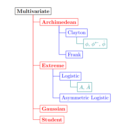The figure shows a object diagram that structures the code. The $\textbf{Multivariate}$ class serves as the root and is used to instantiate all its child classes $\textbf{Archimedean}$, $\textbf{Extreme}$, $\textbf{Gaussian}$, and $\textbf{Student}$ in red. The blue-colored classes correspond to various parametric copula models, and the green-colored classes represent examples of methods. Symbols $\varphi, \varphi^\leftarrow, \dot{\varphi}$ correspond to the generator function, its inverse, and its derivative, respectively, while $A, \dot{A}$ refer to the Pickands dependence function and its derivative.:::The architecture of the code is shown in @fig-diagram. At the third level of the architecture, we find important parametric models of Archimedean and extreme value copulae (depicted as blue in the figure). These parametric models contain methods such as the generator function $\varphi$ (see @sec-arch) for Archimedean copulae and the Pickands dependence function $A$ (see @sec-extreme) for extreme value copulae (depicted as green in the figure). We provide a brief overview of Archimedean copulae and some of their properties in high-dimensional spaces in @sec-arch. A characterization of extreme value copulae is given in @sec-extreme. The from @sec-bv_arch to @sec-mv_ellip define and illustrate all the copula models implemented in the package.## The Archimedean class {#sec-arch}Let $\varphi$ be a generator that is a strictly decreasing, convex function from $[0,1]$ to $[0, \infty]$ such that $\varphi(1) = 0$ and $\varphi(0) = \infty$. We denote the generalized inverse of $\varphi$ by $\varphi^\leftarrow$. Consider the following equation:$$ C(\textbf{u}) = \varphi^\leftarrow (\varphi(u_0)+ \dots + \varphi(u_{d-1})).$$ {#eq-arch_cop}If this relation holds and $C$ is a copula function, then $C$ is called an Archimedean copula. A necessary condition for @eq-arch_cop to be a copula is that the generator $\varphi$ is a $d$-monotonic function, i.e., it is differentiable up to the order $d$ and its derivatives satisfy$$ (-1)^k \left(\varphi\right)^{(k)}(x) \geq 0, \quad k \in \{1, \dots, d\}$$ {#eq-dmono}for $x \in (0, \infty)$ (see Corollary 2.1 of @10.1214/07-AOS556). Note that $d$-monotonic Archimedean inverse generators do not necessarily generate Archimedean copulae in dimensions higher than $d$ (see @10.1214/07-AOS556). As a result, some Archimedean subclasses are only implemented for the bivariate case as they do not generate an Archimedean copula in higher dimensions. In the bivariate case, @eq-dmono can be interpreted as $\varphi$ being a convex function.The $\textsf{clayton}$ package implements common one-parameter families of Archimedean copulae, such as the Clayton (@10.2307/2335289), Gumbel (@1960), Joe (@joe1997multivariate), Frank (@Frank1979), and AMH (@ALI1978405) copulae for the multivariate case. It is worth noting that all Archimedean copulae are symmetric, and in dimensions 3 or higher, only positive associations are allowed. For the specific bivariate case, the package also implements other families, such as those numbered from 4.2.9 to 4.2.15 and 4.2.22 in Section 4.2 of @nelsen2007introduction. Definitions and illustrations of these parametric copula models can be found in @sec-bv_arch and @sec-mv_arch.## The Extreme class {#sec-extreme}Investigating the notion of copulae within the framework of multivariate extreme value theory leads to the extreme value copulae (see @gudendorf2009extremevalue for an overview) defined as $$C(\textbf{u}) = \exp \left( - \ell(-\ln(u_0), \dots, -\ln(u_{d-1})) \right), \quad \textbf{u} \in (0,1]^d,$$ {#eq-evc}where $\ell: [0,\infty)^d \rightarrow [0,\infty)$ the stable tail dependence function which is convex, homogeneous of order one, namely $\ell(c\textbf{x}) = c \ell(\textbf{x})$ for $c > 0$ and satisfies $\max(x_0,\dots,x_{d-1}) \leq \ell(x_0,\dots,x_{d-1}) \leq x_0+\dots+x_{d-1}, \forall \textbf{x} \in [0,\infty)^d$. Let $\Delta^{d-1} = \{\textbf{w} \in [0,1]^d: w_0 + \dots + w_{d-1} = 1\}$ be the unit simplex. The Pickands dependence function $A: \Delta^{d-1} \rightarrow [1/d,1]$ characterizes $\ell$ by its homogeneity, which is the restriction of $\ell$ to the unit simplex $\Delta^{d-1}$:$$ \ell(x_0, \dots,x_{d-1}) = (x_0 + \dots + x_{d-1}) A(w_0, \dots, w_{d-1}), \quad w_j = \frac{x_j}{x_0 + \dots + x_{d-1}},$${#eq-tail_dependence_pickands}for $j \in \{1,\dots,d-1\}$ and $w_0 = 1 - w_1 - \dots - w_{d-1}$ with $\textbf{x} \in [0, \infty)^d \setminus \{\textbf{0}\}$. The Pickands dependence function characterizes the extremal dependence structure of an extreme value random vector and verifies $\max\{w_0,\dots,w_{d-1}\} \leq A(w_0,\dots,w_{d-1}) \leq 1$ where the lower bound corresponds to comonotonicity and the upper bound corresponds to independence. Estimating this function is an active area of research, with many compelling studies having been conducted on the topic (see, for example, @bucher2011new, @GUDENDORF20123073).From a practical point of view, the family of extreme value copulae is very rich and arises naturally as the limiting distribution of properly normalised componentwise maxima. Furthermore, it contains a rich variety of parametric models and allows asymmetric dependence, that is, for the bivariate case:$$ \exists (u_0,u_1) \in [0,1]^2, \quad C(u_0,u_1) \neq C(u_1,u_0).$$In the multivariate framework, the logistic copula (or Gumbel, see @1960), the asymmetric logistic copula (@tawn1990), the Hüsler and Reiss distribution (@HUSLER1989283), the t-EV copula (@Demarta_Mcneil), Bilogistic model (@Smith1990) are implemented. It's worth noting that the logistic copula is the sole model that is both Archimedean and extreme value. The library includes bivariate extreme value copulae such as asymmetric negative logistic (@Joe1990FamiliesOM), asymmetric mixed (@10.1093/biomet/75.3.397). The reader is again invited to read from @sec-bv_ext to @sec-mv_ext for precise definitions of these models.# Random number generator {#sec-rng}We propose a $\textsf{Python}$-based implementation for generating random numbers from a wide variety of copulae. The $\textsf{clayton}$ package requires a few external libraries that are commonly used in scientific computing in $\textsf{Python}$.- `numpy` version 1.6.1 or newer. This is the fundamental package for scientific computing, it contains linear algebra functions and matrix / vector objects (@harris2020array).- `scipy` version 1.7.1 or newer. A library of open-source software for mathematics, science and engineering (@virtanen2020scipy).The $\textsf{clayton}$ package provides two methods for generating random vectors: $\texttt{sample\_unimargin}$ and $\texttt{sample}$. The first method generates a sample where the margins are uniformly distributed on the unit interval $[0,1]$, while the second method generates a sample from the chosen margins.In @sec-biv_case, we present an algorithm that uses the conditioning method to sample from a copula. This method is very general and can be used for any copula that is sufficiently smooth (see @eq-cond_sim and @eq-cond_dist_mv below). However, the practical infeasibility of the algorithm in dimensions higher than $2$ and the computational intensity of numerical inversion call for more efficient ways to sample in higher dimensions. The purpose of @sec-mv_case is to present such methods and to provide details on the methods used in the $\textsf{clayton}$ package. In each section, we provide examples of code to illustrate how to instantiate a copula and how to sample with $\textsf{clayton}$.In the following sections, we will use $\textsf{Python}$ code that assumes that the following packages have been loaded:```{python}import claytonfrom clayton.rng import base, evd, archimedean, monte_carloimport numpy as npimport seaborn as snsimport matplotlib.pyplot as pltfrom scipy.stats import norm, exponplt.style.use('qb-light.mplstyle') # for fancy figuresnp.random.seed(10)```## The bivariate case {#sec-biv_case}In this subsection, we address the problem of generating a bivariate sample from a specified joint distribution with $d=2$. Suppose that we want to sample a bivariate random vector $\textbf{X}$ with copula $C$. In the case where the components are independent, the sampling procedure is straightforward: we can independently sample $X_0$ and $X_1$. However, in the general case where the copula is not the independent copula, this approach is not applicable.One solution to this problem is to use the conditioning method to sample from the copula. This method relies on the fact that given $(U_0, U_1)$ with copula $C$, the conditonal law of $U_1$ given $U_0$ is written as: $$ c_{u_0}(u_1) \triangleq \mathbb{P}\left\{ U_1 \leq u_1 | U_0 = u_0 \right\} = \frac{\partial C(u_0,u_1)}{\partial u_0}.$$ {#eq-cond_sim}This allows us to first sample $U_0$ from a uniform distribution on the unit interval, and then to use the copula to generate $U_1$ given $U_0$. Finally, we can transform the resulting sample $(U_0, U_1)$ into the original space by applying the inverse marginal distributions $F_0^{-1}$ and $F_1^{-1}$ to $U_0$ and $U_1$ respectively. Thus, an algorithm for sampling bivariate copulae is given in @fig-alg-1. Algorithm in @fig-alg-1 presents a procedure for generating a bivariate sample from a copula. The algorithm takes as input the length of the sample $n$, as well as the parameters of the copula ($\theta, \psi_1, \psi_2$). The output is a bivariate sample from the desired copula model, denoted $\{(u_0^{(1)},u_1^{(1)}), \dots, (u_0^{(n)},u_1^{(n)})\}$. This algorithm is applicable as long as the copula has a first partial derivative with respect to its first component.::: {#fig-alg-1}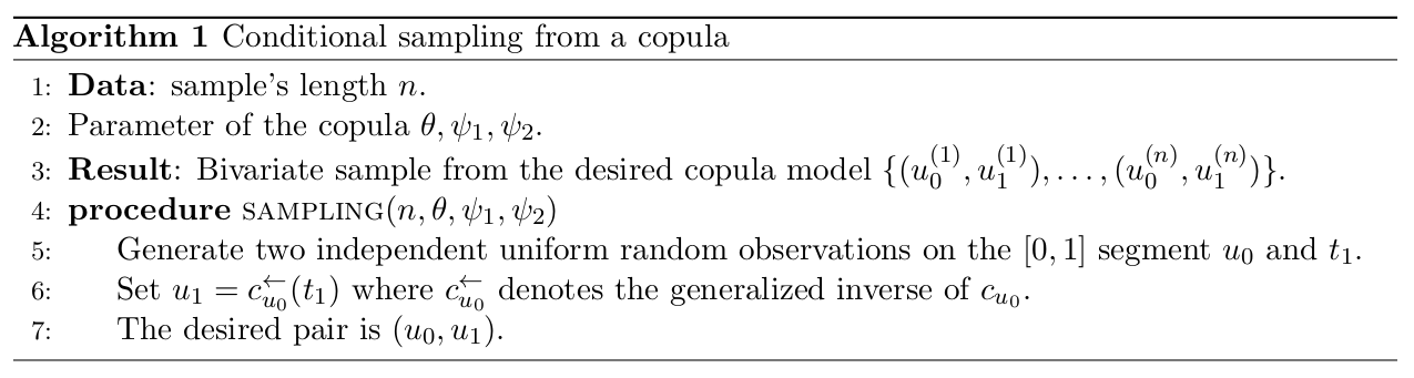Conditional sampling from copula:::For step 6 of the algorithm, we need to find $u_1 \in [0,1]$ such that $c_{u_0}(u_1) - t_1 = 0$ holds. This $u_1$ always exists because for every $u \in ]0,1[$, we have $0 \leq c_{u_0}(u) \leq 1$, and the function $u \mapsto c_{u_0}(u)$ is increasing (see Theorem 2.2.7 of @nelsen2007introduction for a proof). This step can be solved using the \textsf{brentq} function from the \textsf{scipy} package. A sufficient condition for a copula to have a first partial derivative with respect to its first component in the Archimedean and extreme value cases is that the generator $\varphi$ and the Pickands dependence function $A$ are continuously differentiable on $]0,1[$, respectively. In this case, the first partial derivatives of the copula are given by:$$ \frac{\partial C}{\partial u_0}(u_0,u_1) = \frac{\varphi'(u_0)}{\varphi'(C(u_0,u_1))}, \quad (u_0,u_1) \in ]0,1[^2,$$ {#eq-partial_deriv_arch}$$ \frac{\partial C}{\partial u_0}(u_0,u_1) = \frac{\varphi'(u_0)}{\varphi'(C(u_0,u_1))}, \quad (u_0,u_1) \in ]0,1[^2,$$ {#eq-partial_deriv_pick}where $t = \ln(u_1) / \ln(u_0u_1) \in (0,1)$ and $\mu(t) = A(t) - tA'(t)$.We now have all the necessary theoretical tools to give details on how the $\textsf{clayton}$ package is designed. The file $\texttt{base.py}$ contains the $\textbf{Multivariate}$ class and the $\texttt{sample}$ method to generate random numbers from $\textbf{X}$ with copula $C$. To do so, we use the inversion method that is to sample from $\textbf{U}$ using algorithm in @fig-alg-1 and we compose the corresponding uniform margins by $F_j^\leftarrow$. \eqref{eq:cond_sim} indicates that the sole knowledge of $A$ and $\varphi$ and their respective derivatives are needed in order to perform the sixth step of algorithm in @fig-alg-1. For that purpose, $\texttt{cond\_sim}$ method located inside $\textbf{Archimedean}$ and $\textbf{Extreme}$ classes performs algorithm in @fig-alg-1. Then each child of the bivariate $\textbf{Archimedean}$ (resp. $\textbf{Extreme}$) class is thus defined by its generator $\varphi$ (resp. $A$), it's derivative $\varphi'$ (resp. $A'$) and it's inverse $\varphi^\leftarrow$ as emphasized in green in @fig-diagram. Namely, we perform algorithm in @fig-alg-1 for the $\textbf{Archimedean}$ subclasses $\texttt{Frank}$, $\texttt{AMH}$, $\texttt{Clayton}$ (when $\theta < 0$ for the previous three), $\texttt{Nelsen\_9}$, $\texttt{Nelsen\_10}$, $\texttt{Nelsen\_11}$, $\texttt{Nelsen\_12}$, $\texttt{Nelsen\_13}$, $\texttt{Nelsen\_14}$, $\texttt{Nelsen\_15}$ and $\texttt{Nelsen\_22}$. For the $\textbf{Extreme}$ class, such algorithm is performed for the $\texttt{AsyNegLog}$ and $\texttt{AsyMix}$. For other models, faster algorithms are known and thus implemented, we refer to @sec-mv_case for details.The following code illustrates the random vector generation for a bivariate Archimedean copula. By defining the parameter of the copula and the sample's length, the constructor for this copula is available and can be called using the $\texttt{Clayton}$ method, such as:```{python} n_samples, theta =1024, -0.5 copula = archimedean.Clayton(theta=theta, n_samples=n_samples)```To obtain a sample with uniform margins and a Clayton copula, we can use the $\texttt{sample\_unimargin}$ method, as follows:```{python} sample = copula.sample_unimargin()```Here, the $\texttt{sample}$ object is a $\textsf{numpy}$ array with $2$ columns and $1024$ rows, where each row contains a realization from a Clayton copula (see below)```{python} fig, ax = plt.subplots() ax.scatter(sample[:,0], sample[:,1], edgecolors='#6F6F6F', color='#C5C5C5', s=5) ax.set_xlabel(r'$u_0$') ax.set_ylabel(r'$u_1$') plt.show()```## The multivariate case {#sec-mv_case}We will now address the generation of multivariate Archimedean and Extreme value copulae proposed in the Clayton package. In the multivariate case, the link between partial derivatives and the conditional law remains. Indeed, let $(U_0, \dots, U_{d-1})$ be a $d$-dimensional random vector with uniform margins and copula $C$. The conditional distribution of $U_k$ given the values of $U_0, \dots, U_{k-1}$ is$$ \mathbb{P}\left\{ U_k \leq u_k | U_0 = u_0, \dots, U_{k-1} = u_{k-1} \right\} = \frac{\partial^{k-1} C(u_0, \dots, u_k,1,\dots,1)/\partial u_0 \dots \partial u_{k-1}}{\partial^{k-1} C(u_0, \dots, u_{k-1},1,\dots,1) / \partial u_0 \dots \partial u_{k-1}}.$$ {#eq-cond_dist_mv}for $k \in {1,\dots, d-1}$. The conditional simulation algorithm may be written as follows.1. Generate $d$ independent uniform random on $[0,1]$ variates $v_0, \dots, v_{d-1}$.2. Set $u_0 = v_0$.3. For $k = 1, \dots, d-1$, evaluate the inverse of the conditional distribution given by \eqref{eq:cond_dist_mv} at $v_k$, to generate $u_k$.Nevertheless, the evaluation of the inverse conditional distribution becomes increasingly complicated as the dimension $d$ increases. Furthermore, it can be difficult for some models to derive a closed form of @eq-cond_dist_mv that makes it impossible to implement it in a general algorithm with only the dimension $d$ as an input. For multivariate Archimedean copulae, @10.1214/07-AOS556 give a method to generate a random vector from the $d$-dimensional copula $C$ with generator $\varphi$ (see Section 5.2 of @10.1214/07-AOS556). A stochastic representation for Archimedean copulae generated by a $d$-monotone generator is given by$$\textbf{U} = \left( \varphi^\leftarrow(R S_1), \dots, \varphi^\leftarrow(RS_d) \right) \sim C,$$ {#eq-radial}where $R \sim F_R$, the radial distribution which is independent of $S$ and $S$ is distributed uniformly in the unit simplex $\Delta^{d-1}$. One challenging aspect of this algorithm is to have an accurate evaluation of the radial distribution of the Archimedean copula and thus to numerically inverse this distribution. The associated radial distribution for the $\textsf{Clayton}$ copula is given in Example 3.3 @10.1214/07-AOS556 while those of the $\textsf{Joe}$, $\textsf{AMH}$, $\textsf{Gumbel}$ and $\textsf{Frank}$ copulae are given in @hofert2012likelihood. In general, one can use numerical inversion algorithms for computing the inverse of the radial distribution, however it will lead to spurious numerical errors. Other algorithms exist when the generator is known to be the Laplace-Stieltjes transform, denoted as $\mathcal{LS}$, of some positive random variables (see @10.2307/2289314, @frees1998understanding). This positive random variable is often referenced as the frailty distribution. In this framework, Archimedean copulae allow for the stochastic representation$$ \textbf{U} = \left( \varphi^\leftarrow (E_1/V), \dots, \varphi^\leftarrow(E_d /V)\right) \sim C,$$ with $V \sim F = \mathcal{LS}^{-1}[\varphi^\leftarrow]$ the frailty and $E_1, \dots, E_d$ are distributed i.i.d. according to a standard exponential and independent of $V$. Algorithm in @fig-alg-2 presents a procedure for generating a multivariate sample from an Archimedean copula where the frailty distribution is known. The algorithm takes as an input the length of the sample $n$, as well as the parameter of the copula $\theta$. The output is a $d$-variate sample from the desired copula model, denoted $\{(u_0^{(1)}, \dots, u_{d-1}^{(1)}), \dots, (u_0^{(n)},\dots,u_{d-1}^{(n)})\}$.::: {#fig-alg-2}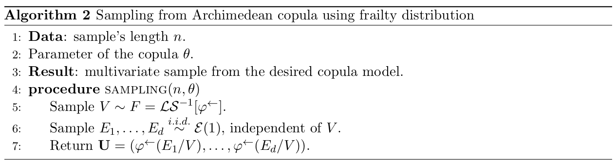Sampling from Archimedean copula using frailty distribution:::In this framework, we define $\texttt{\_frailty\_sim}$ method defined inside the $\textbf{Archimedean}$ class which performs algorithm in @fig-alg-2. Then, each Archimedean copula is defined by the generator $\varphi$, it's inverse $\varphi^\leftarrow$ and the frailty distribution denoted as $\mathcal{LS}^{-1}[\varphi^\leftarrow]$ as long as we know the frailty. This is the case for $\texttt{Joe}$, $\texttt{Clayton}$, $\texttt{AMH}$ or $\texttt{Frank}$.For the extreme value case, algorithms have been proposed, as in @stephenson2003simulating (see Algorithms 2.1 and 2.2), who proposes sampling methods for the Gumbel and the asymmetric logistic model. These algorithms are implemented in the $\textsf{clayton}$ package. Note that these algorithms are model-specific, thus the $\texttt{sample\_unimargin}$ method is exceptionally located in the corresponding child of the multivariate $\textbf{Extreme}$ class. Another procedure designed by @10.1093/biomet/asw008 to sample from multivariate extreme value models using extremal functions (see Algorithm 2 in @10.1093/biomet/asw008) is also of prime interest. For the implemented models using this algorithm, namely $\textbf{Hüsler-Reiss}$, $\textbf{tEV}$, $\textbf{Bilogistic}$ and $\textbf{Dirichlet}$ models, a method called $\texttt{\_rextfunc}$ is located inside each classes which allows to generate an observation from the according law of the extremal function.Samples from the Gaussian and Student copula are directly given by Algorithm 5.9 and 5.10 respectively of @quantrisk. As each algorithm is model specific, the $\texttt{sample\_unimargin}$ method is located inside the $\textbf{Gaussian}$ and $\textbf{Student}$ classes.We present how to construct a multivariate Archimedean copula and to generate random vectors from this model. Introducing the parameters of the copula, we appeal the following lines to construct our copula object:```{python}d, theta, n_samples =3, 2.0, 1024copula = archimedean.Clayton(theta=theta, n_samples=n_samples, dim=d)```We now call the $\texttt{sample\_unimargin}$ method to obtain randomly generated vectors.```{python}sample = copula.sample_unimargin()```We thus represent in three dimensions these realizations below.```{python} fig = plt.figure() ax = fig.add_subplot(111, projection ='3d') ax.scatter3D(sample[:,0], sample[:,1], sample[:,2], s=5, edgecolors='#6F6F6F', color='#C5C5C5') ax.set_xlabel(r'$u_0$') ax.set_ylabel(r'$u_1$') ax.set_zlabel(r'$u_2$') plt.show()```# Case study : Modeling pairwise dependence between spatial maximas with missing data {#sec-pairwise}We now proceed to a case study where we use our \textsf{python} package to assess, under a finite sample framework, the asymptotic properties of an estimator of the $\lambda$-madogram when data are completely missing at random (MCAR). This case study comes from numerical results of @boulin2021non. The $\lambda$-madogram belongs to a family of estimators, namely the madogram, which is of prime interest in environmental sciences, as it is designed to model pairwise dependence between maxima in space, see, e.g., @bernard:hal-03207469, @BADOR201517, @saunders where the madogram was used as a dissimilarity measure to perform clustering. Where in several fields, for example econometrics (@woolridge2007) or survey theory (@chauvet2015), the MCAR hypothesis appears to be a strong hypothesis, this hypothesis is more realistic in environmental research as the missingness of one observation is usually due to instruments, communication and processing errors that may be reasonably supposed independent of the quantity of interest. In @sec-background, we define objects and properties of interest while in @sec-num we describe a detailed tutorial in $\textsf{python}$ and with $\textsf{clayton}$ package to compare the asymptotic variance with an empirical counterpart of the $\lambda$-madogram with $\lambda = 0.5$.## Background {#sec-background}It was emphasized that the possible dependence between maxima can be described with the extreme value copula. This function is completely characterized by the Pickands dependence function (see @eq-tail_dependence_pickands) where the latter is equivalent to the $\lambda$-madogram introduced by @naveau:hal-00312758 and defined as $$ \nu(\lambda) = \mathbb{E}\left[ \left|\{F_0(X_0)\}^{1/\lambda} - \{F_1(X_1)\}^{1/(1-\lambda)} \right|\right],$$ {#eq-lmbd_mado}with $\lambda \in (0,1)$, and if $\lambda = 0$ and $0<u<1$, then $u^{1/\lambda} = 0$ by convention. The $\lambda$-madogram took its inspiration from the extensively used geostatistics tool, the variogram (see Chapter 1.3 of @alma991005826659705596 for a definition and some classical properties). The $\lambda$-madogram can be interpreted as the $L_1$-distance between the uniform margins elevated to the inverse of the corresponding weights $\lambda$ and $1-\lambda$. This quantity describes the dependence structure between extremes by its relation with the Pickands dependence function. If we suppose that $C$ is an extreme value copula as in \eqref{eq:evc}, we have$$ A(\lambda) = \frac{\nu(\lambda) + c(\lambda)}{1-\nu(\lambda) - c(\lambda)},$$ {#eq-pickands_mado}with $c(\lambda) = 2^{-1} (\lambda / (1-\lambda) + (1-\lambda)/\lambda)$ (see Proposition 3 of @MARCON20171 for details).We consider independent and identically distributed i.i.d. copies $\textbf{X}_1, \dots, \textbf{X}_n$ of $\textbf{X}$. In presence of missing data, we do not observe a complete vector $\textbf{X}_i$ for $i \in \{1,\dots,n\}$. We introduce $\textbf{I}_i \in \{0,1\}^2$ which satisfies, $\forall j \in \{0,1\}$, if $X_{i,j}$ is not observed then $I_{i,j} = 0$. To formalize incomplete observations, we introduce the incomplete vector $\tilde{\textbf{X}}_i$ with values in the product space $\bigotimes_{j=1}^2 (\mathbb{R} \cup \{\textsf{NA}\})$ such as$$ \tilde{X}_{i,j} = X_{i,j} I_{i,j} + \textsf{NA} (1-I_{i,j}), \quad i \in \{1,\dots,n\}, \, j \in \{0,\dots, d-1\}.$$We thus suppose that we observe a $4$-tuple such as$$ (\textbf{I}_i, \tilde{\textbf{X}}_i), \quad i \in \{1,\dots,n\},$$ {#eq-missing_2}i.e. at each $i \in \{1,\dots,n\}$, several entries may be missing. We also suppose that for all $i \in \{1, \dots,n \}$, $\textbf{I}_{i}$ are i.i.d copies from $\textbf{I} = (I_0, I_1)$ where $I_j$ is distributed according to a Bernoulli random variable $\mathcal{B}(p_j)$ with $p_j = \mathbb{P}(I_j = 1)$ for $j \in \{0,1\}$. We denote by $p$ the probability of observing completely a realization from $\textbf{X}$, that is $p = \mathbb{P}(I_0=1, I_1 = 1)$. In @boulin2021non, hybrid and corrected estimators, respectively denoted as $\hat{\nu}_n^{\mathcal{H}}$ and $\hat{\nu}_n^{\mathcal{H*}}$, are proposed to estimate nonparametrically the $\lambda$-madogram in presence of missing data completely at random. Furthermore, a closed expression of their asymptotic variances for $\lambda \in ]0,1[$ is also given. This result is summarized in the following proposition.::: {#thm-line}## @boulin2021nonLet $(\textbf{I}_i, \tilde{\textbf{X}_i})_{i=1}^n$ be a samble given by @eq-missing_2. For $\lambda \in ]0,1[$, if $C$ is an extreme value copula with Pickands dependence function $A$, we have as $n \rightarrow \infty$\begin{align*} &\sqrt{n} \left(\hat{\nu}_n^{\mathcal{H}}(\lambda) - \nu( \lambda)\right) \overset{d}{\rightarrow} \mathcal{N}\left(0, \mathcal{S}^{\mathcal{H}}(p_1,p_2,p, \lambda)\right), \\ &\sqrt{n} \left(\hat{\nu}_n^{\mathcal{H}*}(\lambda) - \nu( \lambda)\right) \overset{d}{\rightarrow} \mathcal{N}\left(0, \mathcal{S}^{\mathcal{H}*}(p_1,p_2,p, \lambda)\right),\end{align*}where $\mathcal{S}^{\mathcal{H}}(p_1,p_2,p, \lambda)$ and $\mathcal{S}^{\mathcal{H}*}(p_1,p_2,p, \lambda)$ are the asymptoptic variances of the random variables.:::## Numerical results {#sec-num}Benefiting from generating data with $\textsf{clayton}$ we are thus able, with Monte Carlo simulation, to assess theoretical results given by @thm-line in a finite sample setting. For that purpose, we implement a $\textsf{MonteCarlo}$ class (in $\texttt{monte\_carlo.py}$ file) which contains some methods to perform some Monte Carlo iterations for a given extreme value copula. Now, we set up parameters to sample our bivariate dataset. For this subsection, we choose the asymmetric negative logistic model (see @sec-bv_ext for a definition) with parameters $\theta = 10, \psi_1 = 0.1, \psi_2 = 1.0$ and we define the following function:```{python}def gauss_function(x, x0, sigma):return (np.sqrt(1./ (2*np.pi * sigma**2)) * np.exp(-(x - x0) **2/ (2* sigma**2))) n_samples =512 theta, psi1, psi2 =10, 0.1, 1.0```We choose the standard normal and exponential as margins. To simulate this sample, the following lines should be typed:```{python} copula = evd.AsyNegLog(theta=theta, psi1=psi1, psi2=psi2, n_samples=n_samples) sample = copula.sample(inv_cdf=[norm.ppf, expon.ppf])```The $1024 \times 2$ array $\texttt{sample}$ contains $1024$ realization of the $\textbf{asymmetric negative logistic}$ model where the first column is distributed according to a standard normal random variable and the second column as a standard exponential. This distribution is depicted below. To obtain it, one needs the following lines of command:```{python} fig, ax = plt.subplots() ax.scatter(sample[:,0], sample[:,1], edgecolors="#6F6F6F", color="#C5C5C5", s=5) ax.set_xlabel(r'$x_0$') ax.set_ylabel(r'$x_1$') plt.show()```Before going into further details, we will present the missing mechanism. Let $V_0$ and $V_1$ be random variables uniformly distributed under the $]0,1[$ segment with copula $C_{(V_0,V_1)}$. We set $I_0 = 1\{{V_0 \leq p_0}\}$ and $I_1 = 1\{{V_1 \leq p_1}\}$. It is thus immediate that $I_0 \sim \mathcal{B}(p_0)$ and $I_1 \sim \mathcal{B}(p_1)$ and $p \triangleq \mathbb{P}\{I_0 = 1, I_1 =1 \} = C_{(V_0,V_1)}(p_0, p_1)$. For our illustration, we will take $C_{(V_0,V_1)}$ as a \texttt{Joe} copula with parameter $\theta = 2.0$ (we refer to @sec-bv_arch for a definition of this copula). For this copula, it is more likely to observe a realization $v_0 \geq 0.8$ from $V_0$ if $v_1 \geq 0.8$ from $V_1$. If we observe $v_1 < 0.8$, the realization $v_0$ is close to being independent of $v_1$. In climate studies, extreme events could damage the recording instrument in the surrounding regions where they occur, thus the missingness of one variable may depend on others. We initialize the copula $C_{(V_0,V_1)}$ with the following line:```{python} copula_miss = archimedean.Joe(theta=2.0, n_samples=n_samples)```For a given $\lambda \in ]0,1[$, we now want to estimate a $\lambda$-madogram with a sample from the asymmetric negative logistic model, where some observations are missing due to the missing mechanism described above. We will repeat this step several times to compute an empirical counterpart of the asymptotic variance. The \texttt{MonteCarlo} object has been designed for this purpose: we specify the number of iterations $n_{iter}$ (take $n_{iter} = 1024$), the chosen extreme value copula (asymmetric negative logistic model), the missing mechanism (described by $C_{(V_0,V_1)}$ and $p_0 = p_1 = 0.9$), and $\lambda$ (noted $\texttt{w}$). We can write the following lines of code:```{python} u = np.array([0.9, 0.9]) n_iter, P, w =256, [[u[0], copula_miss._c( u)], [copula_miss._c(u), u[1]]], np.array([0.5,0.5]) monte = monte_carlo.MonteCarlo(n_iter=n_iter, n_samples=n_samples, copula=copula, copula_miss=copula_miss, weight=w, matp=P)```The $\texttt{MonteCarlo}$ object is thus initialized with all parameters needed. We may use the $\texttt{simu}$ method to generate a $\texttt{DataFrame}$ (a $\texttt{pandas}$ object) composed out $1024$ rows and $3$ columns. Each row contains an estimate of the $\lambda$-madogram, $\hat{\nu}_n^{\mathcal{H}*}$ in @thm-line ($\texttt{var\_mado}$), the sample length $n$ ($\texttt{n}$) and the normalized estimation error ($\texttt{scaled}$). We thus call the $\texttt{simu}$ method.```{python} df_wmado = monte.finite_sample(inv_cdf=[norm.ppf, expon.ppf], corr=True)print(df_wmado.head())```The argument $\texttt{corr=True}$ specifies that we compute the corrected estimator, $\hat{\nu}_n^{\mathcal{H}*}$ in @thm-line. Now, using the $\texttt{var\_mado}$ method defined inside in the **Extreme** class, we obtain the asymptotic variance for the given model and parameters from the missing mechanism. We obtain this quantity as follows```{python} var_mado = copula.var_mado(w, jointp=copula_miss._c(u), matp=P, corr=True)print(var_mado)print(df_wmado['scaled'].var())```We propose here to check numerically the asymptotic normality with variance $\mathcal{S}^{\mathcal{H}*}$ of the normalized estimation error of the corrected estimator. We have all data in hand and the asymptotic variance was computed by lines above. We thus write:```{python} sigma = np.sqrt(var_mado) x = np.linspace(min(df_wmado['scaled']), max(df_wmado['scaled']), 1000) gauss = gauss_function(x, 0, sigma) sns.displot(data=df_wmado, x="scaled", color='#C5C5C5', kind='hist', stat='density', common_norm=False, alpha=0.5, fill=True, linewidth=1.5, bins=20) plt.plot(x,gauss, color='#6F6F6F')```# Discussion {#sec-discussion}## Comparison of $\textsf{clayton}$ with $\textsf{R}$ packagesTo compare \textsf{clayton} to existing packages in $\textsf{R}$, we consider the $\textsf{copula}$ package (@kojadinovic2010modeling) and $\textsf{mev}$ (@mevR) for sampling from Archimedean and multivariate extreme value distributions, respectively. To run the experiment, we use two computer clusters. The first cluster consists of five nodes, each with two 18-core Xeon Gold 3.1 GHz processors and 192 GB of memory, with 2933 MHz per socket. The second cluster has two CPU sockets, each containing a Xeon Platinum 8268 2.90 GHz processor with 24 cores. These configurations provide a significant amount of computational power and are well-suited for handling complex, data-intensive tasks. We use the first cluster to install the $\textsf{copula}$ package and sample from the $\textbf{Clayton}$, $\textbf{Frank}$, and $\textbf{Joe}$ models. We consider an increasing dimension $d \in \{50, 100, \dots, 1600\}$ for a fixed sample size of $n=1000$. For the copula package, we compute the average time spent across 100 runs in order to cancel out variability. We use the second cluster to install the $\textsf{mev}$ package and call some of its methods to sample from the $\textbf{Husler Reiss}$, $\textbf{Logistic}$, and $\textbf{TEV}$ distributions. Sampling from the latter is fast, but sampling from the two others is time consuming. Therefore, we only consider dimensions $d \in \{25, 50, \dots, 250\}$ for a fixed sample size of $n=1000$.::: {#fig-num_res layout-ncol=2}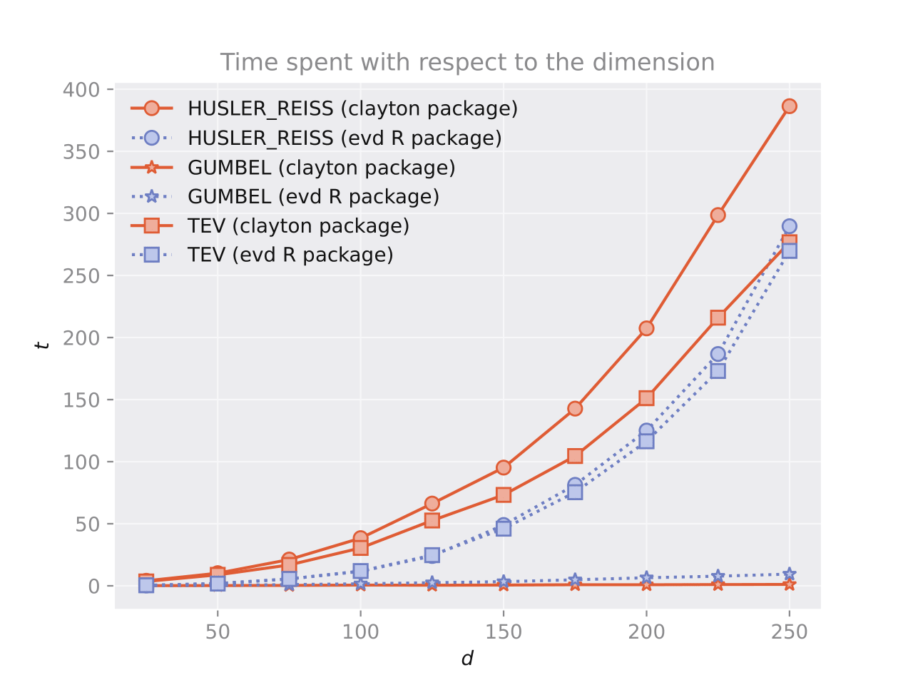Comparison results. Time spent (in seconds) to sample from the corresponding models with respect to the dimension $d$. The left panel shows the results for sampling from $\textbf{Clayton}$, $\textbf{Frank}$ and $\textbf{Joe}$ using $\textsf{clayton}$ in $\textsf{Python}$ and $\textsf{copula}$ in $\textsf{R}$. The right panel shows the results for sampling from $\textbf{HuslerReiss}$, $\textbf{Logistic}$ and $\textbf{TEV}$ by $\textsf{clayton}$ in $\textsf{Python}$ and $\textsf{mev}$ in $\textsf{R}$. In both cases, $1000$ vectors are generated for each model.:::The figure shows the results of a comparison between the $\textsf{clayton}$ and $\textsf{copula}$ packages in $\textsf{R}$, and the $\textsf{mev}$ package in $\textsf{Python}$. The comparison shows that the $\textsf{clayton}$ package is more efficient at sampling from $\textbf{Clayton}$, $\textbf{Frank}$ and $\textbf{Joe}$ copulae than the $\textsf{copula}$ package. The gap in efficiency may be due to the choice of algorithms used in the $\textsf{clayton}$ package, which uses frailty distributions. The time required for sampling increases linearly with the dimension for the $\textsf{clayton}$ package, but shows a more erratic behavior for the $\textsf{copula}$ package.## ConclusionThis paper presents the construction and some implementations of the $\textsf{Python}$ package $\textsf{clayton}$ for random copula sampling. This is a seminal work in the field of software implementation of copula modeling in $\textsf{Python}$ and there is much more potential for growth. It is hoped that the potential diffusion of the software through those who need it may bring further implementations for multivariate modeling with copulae under $\textsf{Python}$. For example, choosing a copula to fit the data is an important but difficult problem. A robust approach to estimating copulae has been investigated recently by @alquier2020estimation using Maximum Mean Discrepancy. In relation to our example, semiparametric estimation of copulae with missing data could be of great interest, as proposed by @HAMORI201985.Additionally, implementation of the algorithm proposed by @10.1214/07-AOS556 for generating random vectors for Archimedean copulae has been tackled, but as expected, numerical inversion gives spurious results, especially when the parameter $\theta$ and the dimension $d$ are high. Furthermore, as the support of the radial distribution is contained in the real line, numerical inversion leads to increased computational time. Further investigation is needed in order to generate random vectors from classical Archimedan models using the radial distribution.A direction of improvement for the $\textsf{clayton}$ package is dependence modeling with Vine copulae, which have recently been a tool of high interest in the machine learning community (see, e.g., @lopez2013gaussian, @Veeramachaneni2015CopulaGM, @Carrera2016VineCC, @10.5555/2946645.2946678 or @SunCuesta-InfanteVeeramachaneni2019). This highlights the need for dependence modeling with copulae in $\textsf{Python}$, as a significant part of the machine learning community uses this language. In relation to this paper, Vine copulae may be useful for modeling dependencies between extreme events, as suggested by @SIMPSON2021104736, @nolde2021linking. Furthermore, other copula models could be implemented to model further dependencies. These implementations will expand the scope of dependence modeling with $\textsf{Python}$ and provide high-quality, usable tools for anyone who needs them.# References {.unnumbered}::: {#refs}:::# Appendix {#appendices}## Bivariate Archimedean models {#sec-bv_arch}::: {#fig-bv_arch-1}{width=100%}:::::: {#fig-bv_arch-2}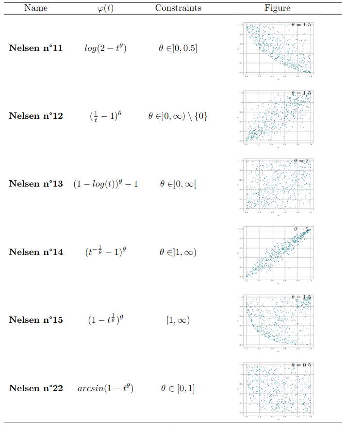{width=100%}:::## Implemented bivariate extreme models {#sec-bv_ext}::: {#fig-bv-ext}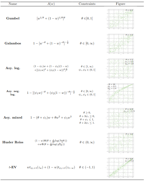{width=100%}:::## Multivariate Archimedean copulae {#sec-mv_arch}::: {#fig-mv-arch}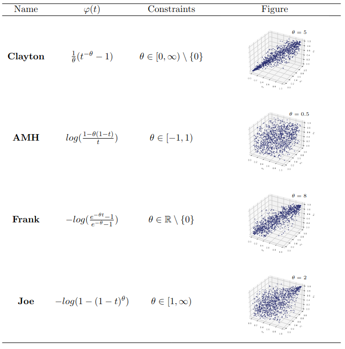{width=100%}:::## Multivariate extreme models {#sec-mv_ext}Before giving the main details, we introduce some notations. Let $B$ be the set of all nonempty subsets of $\{1,\dots,d\}$ and $B_1 = \{b \in B, |b| = 1\}$, where $|b|$ denotes the number of elements in thet set $b$. We note by $B_{(j)} = \{b \in B, j \in b\}$. For $d=3$, the Pickands is expressed as::: {#eq-mv_ext}\begin{align*} A(\textbf{w}) =& \alpha_1 w_1 + \psi_1 w_2 + \phi_1 w_3 + \left( (\alpha_2 w_1)^{\theta_1} + (\psi_2w_2)^{\theta_1} \right)^{1/\theta_1} + \left( (\alpha_3 w_2)^{\theta_2} + (\phi_2w_3)^{\theta_2} \right)^{1/\theta_2} \\ &+ \left( (\psi_3 w_2)^{\theta_3} + (\phi_3w_3)^{\theta_3} \right)^{1/\theta_3} + \left( (\alpha_4 w_1)^{\theta_4} + (\psi_4 w_2)^{\theta_4} + (\phi_4 w_3)^{\theta_4} \right)^{1/\theta_4},\end{align*}::: where $\boldsymbol{\alpha} = (\alpha_1, \dots, \alpha_4), \boldsymbol{\psi} = (\psi_1, \dots, \psi_4), \boldsymbol{\phi} = (\phi_1, \dots, \phi_4)$ are all elements of $\Delta^3$. We take $\boldsymbol{\alpha} = (0.4,0.3,0.1,0.2)$, $\boldsymbol{\psi} = (0.1, 0.2, 0.4, 0.3)$, $\boldsymbol{\phi} = (0.6,0.1,0.1,0.2)$ and $\boldsymbol{\theta} = (\theta_1, \dots, \theta_4) = (0.6,0.5,0.8,0.3)$ as the dependence parameter.The Dirichlet model is a mixture of $m$ Dirichlet densities, that is$$ h(\textbf{w}) = \sum_{k=1}^m \theta_k \frac{\Gamma(\sum_{j=1}^d \sigma_{kj})}{\Pi_{j=1}^d \Gamma(\sigma_{kj})} \Pi_{j=1}^d w_j^{\sigma_{kj}-1},$$with $\sum_{k=1}^m \theta_k = 1$, $\sigma_{kj} > 0$ for $k \in \{1,\dots,m\}$ and $j \in \{1, \dots, d\}$. Let $\mathcal{D} \in [0, \infty)^{(d-1)\times (d-1)}$ denotes the space of symmetric strictly conditionnaly negative definite matrices that is::: {#striclty_cond_neg}\begin{align*} \mathcal{D}_{k} = \Big\{ \Gamma \in [0,\infty)^{k \times k} : a^\top \Gamma a < 0 \; \textrm{for all } a \in \mathbb{R}^{k} \setminus \{\textbf{0}\} \, \textrm{with } \sum_{j=1}^{d-1} a_j = 0, \\ \Gamma_{ii} = 0, \Gamma_{ij} = \Gamma_{ji}, \quad 1 \leq i,j\leq k \Big\}. \end{align*}::: For any $2 \leq k \leq d$, consider $m' = (m_1, \dots, m_k)$ with $1 \leq m_1 < \dots < m_k \leq d$ define$$ \Sigma^{(k)}_m = 2 \left( \Gamma_{m_i m_k} + \Gamma_{m_j m_k} - \Gamma_{m_i m_j} \right)_{m_i m_j \neq m_k} \in [0,\infty)^{(d-1)\times(d-1)}.$$Furthermore, note $S(\cdot | \Sigma^{(k)}_m)$ denote the survival function of a normal random vector with mean vector $\textbf{0}$ and covariance matrix $\Sigma^{(k)}$. We now define :$$ h_{km}(\textbf{y}) = \int_{y_k}^\infty S\left( (y_i - z + 2\Gamma_{m_i m_k})_{i=1}^{k-1} | \Gamma_{km}\right) e^{-z}dz $$for $2 \leq k \leq d$. We denote by $\Sigma^{(k)}$ the summation over all $k$-vectors $m=(m_1,\dots,m_k)$ with $1\leq m_1 < \dots < m_k \leq d$.::: {#fig-mv_ext}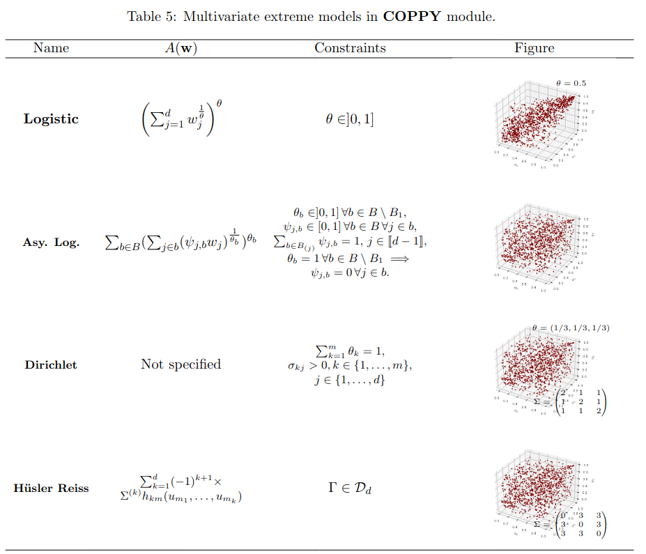{width=100%}:::## Multivariate elliptical dependencies {#sec-mv_ellip}Let $\textbf{X} \sim \textbf{E}_d(\boldsymbol{\mu}, \Sigma, \psi)$ be an elliptical distributed random vector with cumulative distribution $F$ and marginal $F_0, \dots, F_{d-1}$. Then, the copula $C$ of $F$ is called an elliptical copula. We denote by $\phi$ the standard normal distribution function and $\boldsymbol{\phi}_\Sigma$ the joint distribution function of $\textbf{X} \sim \mathcal{N}_d(\textbf{0}, \Sigma)$, where $\textbf{0}$ is the $d$-dimensional vector composed out of $0$. In the same way, we note $t_{\theta}$ the distribution function of a standard univariate distribution $t$ distribution and by $\boldsymbol{t}_{\theta, \Sigma}$ the joint distribution function of the vector $\textbf{X} \sim \boldsymbol{t}_{d}(\theta, \textbf{0}, \Sigma)$. A $d$ squared matrix $\Sigma$ is said to be positively semi definite if for all $u \in \mathbb{R}^d$ we have :$$ u^\top \Sigma u \geq 0$$::: {#fig-mv_elli}{width=100%}:::


